[논문리뷰] Sharpness-Aware Minimization for Efficiently Improving Generalization
ICLR 2021. [Paper] [Github]
Pierre Foret, Ariel Kleiner, Hossein Mobahi, Behnam Neyshabur
Google Research | Blueshift, Alphabet
3 Oct 2020
Introduction
본 논문에서는 loss 값과 loss sharpness를 동시에 최소화하여 모델 일반화 성능을 향상시키는 새로운 방법인 Sharpness-Aware Minimization (SAM)을 소개한다. SAM은 loss 값이 낮은 파라미터만을 찾는 것이 아니라, loss 값이 균일하게 낮은 주변 영역에 있는 파라미터를 찾는 방식으로 작동한다. 또한 효율적이고 쉽게 구현할 수 있다.
SAM을 사용하면 널리 연구되어 온 다양한 컴퓨터 비전 task 및 모델에서 모델의 일반화 능력이 향상된다. 또한, SAM은 noisy label 환경을 특별히 겨냥해서 만든 SOTA 기법과 비슷한 수준의 robustness를 제공한다.
Method
분포 $\mathcal{D}$에서 독립적으로 추출된 학습 데이터셋 \(\mathcal{S} = \bigcup_{i=1}^n (\{\textbf{x}_i, \textbf{y}_i\})\)가 주어졌을 때, 본 논문의 목표는 일반화 성능이 우수한 모델을 학습하는 것이다. 특히, 파라미터 $\textbf{w}$를 갖는 모델을 고려할 때, 데이터 포인트별 loss function $l$이 주어지면, 학습 데이터셋 loss \(L_\mathcal{S} (\textbf{w})\)와 모집단 loss \(L_\mathcal{D} (\textbf{w})\)를 다음과 같이 정의한다.
\[\begin{equation} L_\mathcal{S} (\textbf{w}) = \frac{1}{n} \sum_{i=1}^n l (\textbf{w}, \textbf{x}_i, \textbf{y}_i), \quad L_\mathcal{D} (\textbf{w}) = \mathbb{E}_{(\textbf{x}, \textbf{y}) \sim \mathcal{D}} [l(\textbf{w}, \textbf{x}, \textbf{y})] \end{equation}\]모델 학습의 목표는 관찰된 데이터셋 $\mathcal{S}$만을 사용하여 모집단 loss \(L_\mathcal{D} (\textbf{w})\)가 낮은 모델 파라미터 $\textbf{w}$를 선택하는 것이다. 안타깝게도 현대 모델에서 \(L_\mathcal{S} (\textbf{w})\)는 일반적으로 $\textbf{w}$에 대하여 non-convex function이며, 유사한 \(L_\mathcal{S} (\textbf{w})\)를 가지면서도 일반화 성능, 즉 상당히 다른 \(L_\mathcal{D}\)를 보이는 여러 local minima 또는 global minima를 가질 수 있다.
Loss landscape가 날카로울수록 일반화 능력이 향상된다는 점에 착안하여, 본 논문에서는 다른 접근 방식을 제안하였다. 단순히 \(L_\mathcal{S} (\textbf{w})\)가 낮은 파라미터 $\textbf{w}$를 찾는 대신, 주변 영역 전체가 균일하게 낮은 학습 loss 값을 갖는 파라미터, 즉 loss 값과 곡률이 모두 낮은 영역을 찾는 것이다.
분포 $\mathcal{D}$에서 생성된 $\mathcal{S}$에 대해 높은 확률로, 임의의 $\rho > 0$에 대해, 다음 정리가 성립한다.
\[\begin{equation} L_\mathcal{D} (\textbf{w}) \le \max_{\| \boldsymbol{\epsilon} \|_2 \le \rho} L_\mathcal{S} (\textbf{w} + \boldsymbol{\epsilon}) + h(\| \textbf{w} \|_2^2 / \rho^2) \end{equation}\]($h: \mathbb{R}^{+} \rightarrow \mathbb{R}^{+}$는 strictly increasing function)
Sharpness 항을 명확히 하기 위해 위 부등식의 우변을 다음과 같이 다시 쓸 수 있다.
\[\begin{equation} [\max_{\| \boldsymbol{\epsilon} \|_2 \le \rho} L_\mathcal{S} (\textbf{w} + \boldsymbol{\epsilon}) - L_\mathcal{S} (\textbf{w})] + L_\mathcal{S} (\textbf{w}) + h(\| \textbf{w} \|_2^2 / \rho^2) \end{equation}\]대괄호 안의 항은 $\textbf{w}$에서 \(L_\mathcal{S}\)의 sharpness를 나타내며, $\textbf{w}$에서 인접한 파라미터 값으로 이동할 때 학습 loss가 얼마나 빠르게 증가하는지를 측정한다. 이 sharpness 항은 \(L_\mathcal{S}\) 값 자체와 $\textbf{w}$의 크기에 대한 정규화 항과 합산된다. $h$는 \(\lambda \| \textbf{w} \|_2^2\)로 대체한다.
따라서, 저자들은 다음과 같은 SharpnessAware Minimization (SAM) 문제를 해결하여 파라미터 값을 선택하는 방법을 제안하였다.
\[\begin{equation} \min_\textbf{w} L_\mathcal{S}^\textrm{SAM} (\textbf{w}) + \lambda \| \textbf{w} \|_2^2 \quad \textrm{where} \quad L_\mathcal{S}^\textrm{SAM} (\textbf{w}) = \max_{\| \boldsymbol{\epsilon} \|_2 \le \rho} L_\mathcal{S} (\textbf{w} + \boldsymbol{\epsilon}) \end{equation}\]($\rho$와 $\lambda$는 hyperparameter)
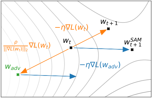
\(L_\mathcal{S}^\textrm{SAM} (\textbf{w})\)를 최소화하기 위해, inner maximization을 통해 미분함으로써 \(\nabla_\textbf{w} L_\mathcal{S}^\textrm{SAM} (\textbf{w})\)에 대한 효율적이고 효과적인 근사치를 도출할 수 있다. 이를 통해 stochastic gradient descent (SGD)를 SAM loss에 직접 적용할 수 있다. 먼저, $\textbf{0}$ 주변의 \(\boldsymbol{\epsilon}\)에 대한 \(L_\mathcal{S} (\textbf{w} + \boldsymbol{\epsilon})\)의 1차 테일러 전개를 통해 inner maximization 문제를 근사화하여 다음을 얻는다.
\[\begin{aligned} \boldsymbol{\epsilon}^\ast (\textbf{w}) &= \underset{\| \boldsymbol{\epsilon} \|_2 \le \rho}{\arg \max} L_\mathcal{S} (\textbf{w} + \boldsymbol{\epsilon}) \\ &\approx \underset{\| \boldsymbol{\epsilon} \|_2 \le \rho}{\arg \max} L_\mathcal{S} (\textbf{w}) + \boldsymbol{\epsilon}^\top \nabla_\textbf{w} L_\mathcal{S} (\textbf{w}) \\ &= \underset{\| \boldsymbol{\epsilon} \|_2 \le \rho}{\arg \max} \boldsymbol{\epsilon}^\top \nabla_\textbf{w} L_\mathcal{S} (\textbf{w}) \end{aligned}\]이 근사치를 만족하는 값 \(\hat{\boldsymbol{\epsilon}} (\textbf{w})\)는 고전적인 dual norm problem의 해로 주어진다.
\[\begin{equation} \hat{\boldsymbol{\epsilon}} (\textbf{w}) = \rho \frac{\nabla_\textbf{w} L_\mathcal{S} (\textbf{w})}{\| \nabla_\textbf{w} L_\mathcal{S} (\textbf{w}) \|_2} \end{equation}\]다시 대입하고 미분하면 다음과 같다.
\[\begin{aligned} \nabla_\textbf{w} L_\mathcal{S}^\textrm{SAM} (\textbf{w}) &\approx \nabla_\textbf{w} L_\mathcal{S}(\textbf{w} + \hat{\boldsymbol{\epsilon}}(\textbf{w})) = \frac{d (\textbf{w} + \hat{\boldsymbol{\epsilon}}(\textbf{w}))}{d \textbf{w}} \nabla_\textbf{w} L_\mathcal{S} (\textbf{w}) \vert_{\textbf{w} + \hat{\boldsymbol{\epsilon}}(\textbf{w})} \\ &= \nabla_\textbf{w} L_\mathcal{S}(\textbf{w}) \vert_{\textbf{w} + \hat{\boldsymbol{\epsilon}}(\textbf{w})} + \frac{d \hat{\boldsymbol{\epsilon}}(\textbf{w})}{d \textbf{w}} \nabla_\textbf{w} L_\mathcal{S} (\textbf{w}) \vert_{\textbf{w} + \hat{\boldsymbol{\epsilon}}(\textbf{w})} \end{aligned}\]\(\nabla_\textbf{w} L_\mathcal{S}^\textrm{SAM} (\textbf{w})\)에 대한 이 근사값은 JAX, TensorFlow, PyTorch와 같은 일반적인 라이브러리에 구현된 자동 미분을 통해 간단하게 계산할 수 있다. \(\hat{\boldsymbol{\epsilon}} (\textbf{w})\) 자체가 \(\nabla_\textbf{w} L_\mathcal{S}(\textbf{w})\)의 함수이기 때문에 이 계산은 \(L_\mathcal{S}(\textbf{w})\)의 Hessian에 의존하지만, Hessian은 Hessian을 직접 생성하지 않고도 계산 가능한 Hessian-vector product을 통해서만 나타난다. 그럼에도 불구하고 계산 속도를 더욱 높이기 위해 2차 항을 제거하여 최종 gradient 근사값을 얻는다.
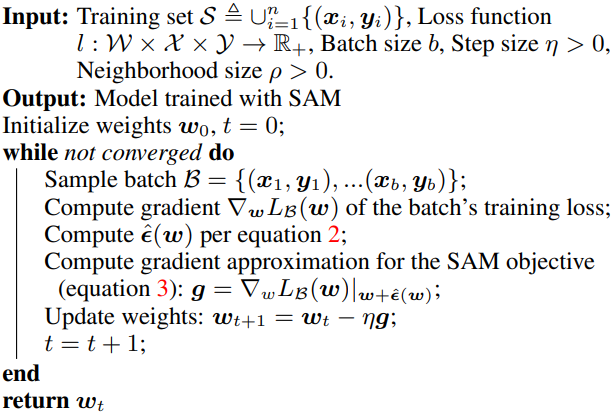
\[\begin{equation} \nabla_\textbf{w} L_\mathcal{S}^\textrm{SAM} (\textbf{w}) \approx \nabla_\textbf{w} L_\mathcal{S}(\textbf{w}) \vert_{\textbf{w} + \hat{\boldsymbol{\epsilon}}(\textbf{w})} \end{equation}\]저자들은 SGD와 같은 표준 optimizer를 SAM loss \(L_\mathcal{S}^\textrm{SAM} (\textbf{w})\)에 적용하고, 위 식을 이용하여 필요한 gradient를 계산한다. 아래는 SGD를 기본 optimizer로 사용하는 전체 SAM 알고리즘이다.
Experiments
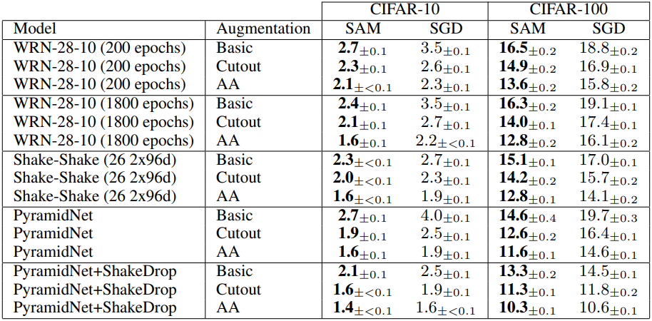
1. Image Classification From Scratch
다음은 CIFAR-10과 CIFAR-100에 대한 test error rate를 비교한 결과이다.
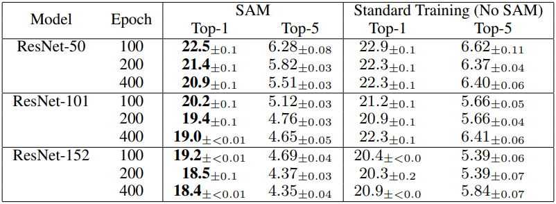
다음은 ImageNet에서 학습된 ResNet에 대한 test error rate를 SAM 적용 유무에 대하여 비교한 결과이다.
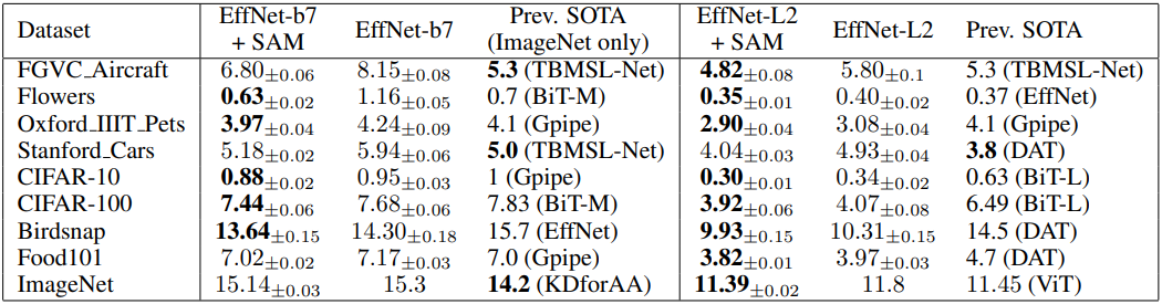
2. Finetuning
다음은 EfficientNet-b7과 EfficientNet-L2를 finetuning한 모델에 대한 top-1 error rate를 비교한 결과이다.
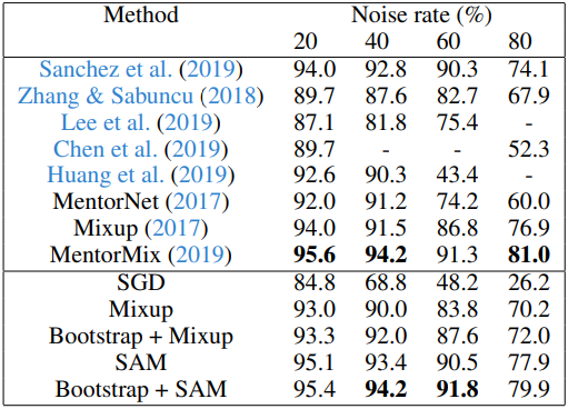
3. Robustness to Label Noise
다음은 noisy label로 학습된 모델의 CIFAR-10 성능을 비교한 결과이다.