[논문리뷰] Bayesian-LoRA: Probabilistic Low-Rank Adaptation of Large Language Models

ICML 2026. [Paper]
Moule Lin, Shuhao Guan, Andrea Patane, David Gregg, Goetz Botterweck
Trinity College Dublin
28 Jan 2026

Introduction

LLM을 fine-tuning하는 데 있어, Low-Rank Adaptation (LoRA)와 같은 파라미터 효율적인 방법을 사용하는 것이 표준 관행이 되었다. 사전 학습된 모델은 기본적으로 calibration, 즉 확률적 신뢰도 정렬이 상당히 잘 되어 있지만, 도메인별 fine-tuning을 거치면 calibration 상태가 종종 저하되고 결과적으로 모델이 과신하는 경향이 있다. 따라서 LLM 학습 중에 확률 calibration을 유지하거나 개선할 수 있는 calibration-aware fine-tuning 방법이 필요하다. 그러나 완전한 Bayesian inference는 LLM 규모에서 계산적으로 불가능하며, Laplace 방법과 같은 효율적인 근사법은 학습 후 calibration를 수정한다.

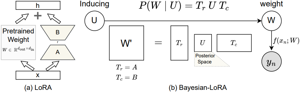
Sparse Gaussian Process (SGP) inference에서 Kronecker-factorized conditional distribution은 가중치 업데이트 $M_W(U) = T_r U T_c$를 생성하는데, 이는 full matrix를 직접 업데이트하지 않고 factorized form으로 업데이트를 제한한다는 점에서 LoRA와 구조적으로 대응된다. 본 논문에서는 이러한 관찰에서 파생된 calibration-aware fine-tuning 프레임워크인 Bayesian-LoRA를 제안하였다.

$T_r$, $T_c$는 LoRA의 $B$, $A$ 행렬과 유사한 역할을 하며, inducing matrix $U$는 가중치 업데이트를 확률적으로 만든다. 이는 LoRA가 확률적 프레임워크 내에 자연스럽게 포함될 수 있으며, deterministic한 LoRA는 극한 사례로 나타난다.

$U$에 대한 non-degenerate variational posterior를 유지하고, 이를 normalizing flow로 강화함으로써, calibration된 불확실성을 갖는 확률적 일반화를 얻는다. 이 설계는 세 가지 장점을 제공한다.

1. 불확실성이 low-rank inducing space에서 모델링되므로 오버헤드가 최소화된다.
2. Closed-form KL 항을 사용하므로 비용이 많이 드는 Hessian 계산을 피할 수 있다.
3. Calibration이 학습 과정에서 end-to-end로 최적화된다.

Method

1. Variational Sparse Inducing Weight Model

핵심 아이디어

\(W \in \mathbb{R}^{d_\textrm{out} \times d_\textrm{in}}\)에 직접 분포를 적용하는 대신, \(r \ll d_\textrm{out}\), \(c \ll d_\textrm{in}\)인 간결한 inducing matrix $U \in \mathbb{R}^{r \times c}$를 도입하여 $W$에 대한 분포를 제어한다. Sparse Gaussian Process (SGP)에서와 마찬가지로, 저차원 행렬 $U$는 $W$에 대한 posterior에 대해 충분한 통계량 역할을 하여 inference를 다루기 쉽게 만든다.

$U$에 대한 prior와 variational posterior

$U$에 Gaussian (matrix-normal) prior를 적용한다.

\[\begin{equation} p(U) = \mathcal{N} (\textrm{vec}(U) \mid \textbf{0}, K_U), \quad K_U = K_c \otimes K_r \end{equation}\]

($K_r \in \mathbb{R}^{r \times r}$과 $K_c \in \mathbb{R}^{c \times c}$는 학습 가능한 covariance factor, $\otimes$는 Kronecker product)

Variational posterior는 다음과 같다.

\[\begin{equation} q(U) = \mathcal{N} (\textrm{vec} (U) \mid \textbf{m}, \textbf{S}) \end{equation}\]

주어진 $U$에 대한 $W$의 조건부 분포

주어진 $U$에 대해, 가중치 행렬 $W$는 조건부 Gaussian 분포을 따른다.

\[\begin{equation} p(W \mid U) = \mathcal{N} (W \mid M_W (U), \lambda^2 \Sigma_W) \end{equation}\]

($\lambda$는 학습 가능한 scale 파라미터)

Covariance factor는 다음과 같이 parameterize된다.

\[\begin{equation} K_r = Z_r Z_r^\top + D_r^2, \quad K_r = Z_c Z_c^\top + D_c^2 \end{equation}\]

($Z_r \in \mathbb{R}^{r \times r}$과 $Z_c \in \mathbb{R}^{c \times c}$는 학습 가능한 행렬, $D_r$, $D_c$는 diagonal noise matrix)

다음과 같은 projection 연산자 $T_r$, $T_c$로 $W$의 조건부 평균을 bilinear projection으로 정의한다.

\[\begin{equation} T_r = Z_r^\top K_r^{-1}, \quad T_c = K_c^{-1} Z_c \\ M_W (U) = T_r U T_c \end{equation}\]

Marginal distribution과 ELBO

$W$에 대한 marginal distribution은 $U$에 대한 적분으로 얻을 수 있다.

\[\begin{equation} q(W) = \int p (W \mid U) p(U) dU \end{equation}\]

따라서 $U$의 저차원 파라미터만 최적화하면 $W$에 대한 고차원 posterior를 근사화하기에 충분하다. ELBO는 다음과 같은 형태를 취한다.

\[\begin{equation} \mathcal{L} = \mathbb{E}_{q(W)} \left[ \log p (\mathcal{D} \mid W) \right] - \textrm{KL} \left( q(U) \; \| \; p(U) \right) - \mathbb{E}_{q(U)} \left[ \textrm{KL} \left( q(W \mid U) \; \| \; p(W \mid U) \right) \right] \end{equation}\]

2. From LoRA to Bayesian-LoRA

확률적 low-rank 업데이트

LoRA는 deterministic한 rank-$r$ 업데이트를 사용한다.

\[\begin{equation} \Delta W_\textrm{LoRA} = \frac{\alpha}{r} BA, \quad B \in \mathbb{R}^{d_\textrm{out} \times r}, \; A \in \mathbb{R}^{r \times d_\textrm{out}} \end{equation}\]

Bayesian-LoRA에서는 이를 확률적 업데이트로 대체한다. 각 layer에 대해 저차원 inducing matrix $U \in \mathbb{R}^{r \times c}$를 도입하고 conditional Gaussian $p(W \mid U)$를 통해 해당 정보를 고차원 가중치 공간으로 확산시킨다. $M_W(U) = T_r U T_c$는 LoRA 행렬 $A$와 $B$의 확률적 유사체 역할을 한다. $U$의 각 몬테카를로 샘플은 서로 다른 가중치를 생성하며, 이러한 분포는 불확실성을 인코딩한다.

Posterior 유연성을 위한 normalizing flow

$U$에 대한 순수한 Gaussian posterior는 LLM의 가중치 공간 불확실성을 포착하는 데 너무 제한적일 수 있다. 따라서 저자들은 diagonal-Gaussian base distribution 위에 normalizing flow를 배치하여, 파라미터 개수를 적게 유지하면서 근사 posterior로 표현할 수 있는 분포의 형태를 더 다양하고 유연하게 만들었다.

\[\begin{aligned} q_0 (U_0) &= \mathcal{N} (\textrm{vec}(U_0) \mid \textbf{m}, \textrm{diag}(\boldsymbol{\sigma}^2)), \quad \boldsymbol{\sigma} \in \mathbb{R}_{> 0}^{rc} \\ U &= T_\phi (U_0) \end{aligned}\]

여기서 \(T_\phi\)는 가역적이고 미분 가능한 매핑이며, 실제로는 가벼운 row-wise Masked Autoregressive Flow (MAF)를 사용한다. Flow 용량을 증가시키면 posterior 표현력과 calibration이 향상된다.

3. Training Objective: Flow-Augmented ELBO

Change-of-variables 공식을 이용하면 $U$의 밀도는 다음과 같다.

\[\begin{equation} \log q_\phi (U) = \log q_0 \left( T_\phi^{-1}(U) \right) - \log \left\vert \textrm{det} J_{T_\phi} \left( T_\phi^{-1}(U) \right) \right\vert \end{equation}\]

\(q_\phi (U)\)를 ELBO 식에 대입하고 정리하면 다음과 같다.

\[\begin{equation} \mathcal{L} = \mathbb{E}_{U_0 \sim q_0, \epsilon} \left[ \log p (\mathcal{D} \mid W) \right] - \mathbb{E}_{U_0 \sim q_0} \left[ \log q_0 (U_0) - \log \vert \textrm{det} J_{T_\phi} (U_0) \vert - \log p \left( T_\phi (U_0) \right) \right] - \frac{D}{2} \left( \lambda^2 - 1 - 2 \log \lambda \right) \\ \textrm{where} \quad D = \sum_\ell d_W^{(\ell)}, \quad d_W^{(\ell)} = d_\textrm{out}^{(\ell)} d_\textrm{in}^{(\ell)} \end{equation}\]

Jacobian determinant \(\log \vert \textrm{det} J_{T_\phi} (U_0) \vert\)는 MAF의 autoregressive한 구조에 의해 효율적으로 계산된다.

LoRA와의 구조적 동형성

조건부 평균 $M_W(U) = T_r U T_c$는 공유된 bilinear function 형태의 의미에서 LoRA의 $\Delta W = \frac{\alpha}{r} BA$와 구조적 동형성을 나타낸다. $T_r$은 $B$와 유사한 역할을 하고, $T_c$는 $A$와 유사한 역할을 하며, $U$는 deterministic한 행렬 곱을 확률적으로 만든다. $r = c$인 경우, Bayesian-LoRA는 불확실성 정량화를 추가하면서 LoRA와 동일한 low-rank subspace에서 가중치 업데이트를 생성한다. 표준 LoRA는 $(A, B)$를 파라미터로 직접 최적화하는 반면, Bayesian-LoRA는 공분산 구조에서 파생된 $T_r$, $T_c$를 사용하여 U를 최적화한다.

Experiments

1. In-Distribution Evaluation

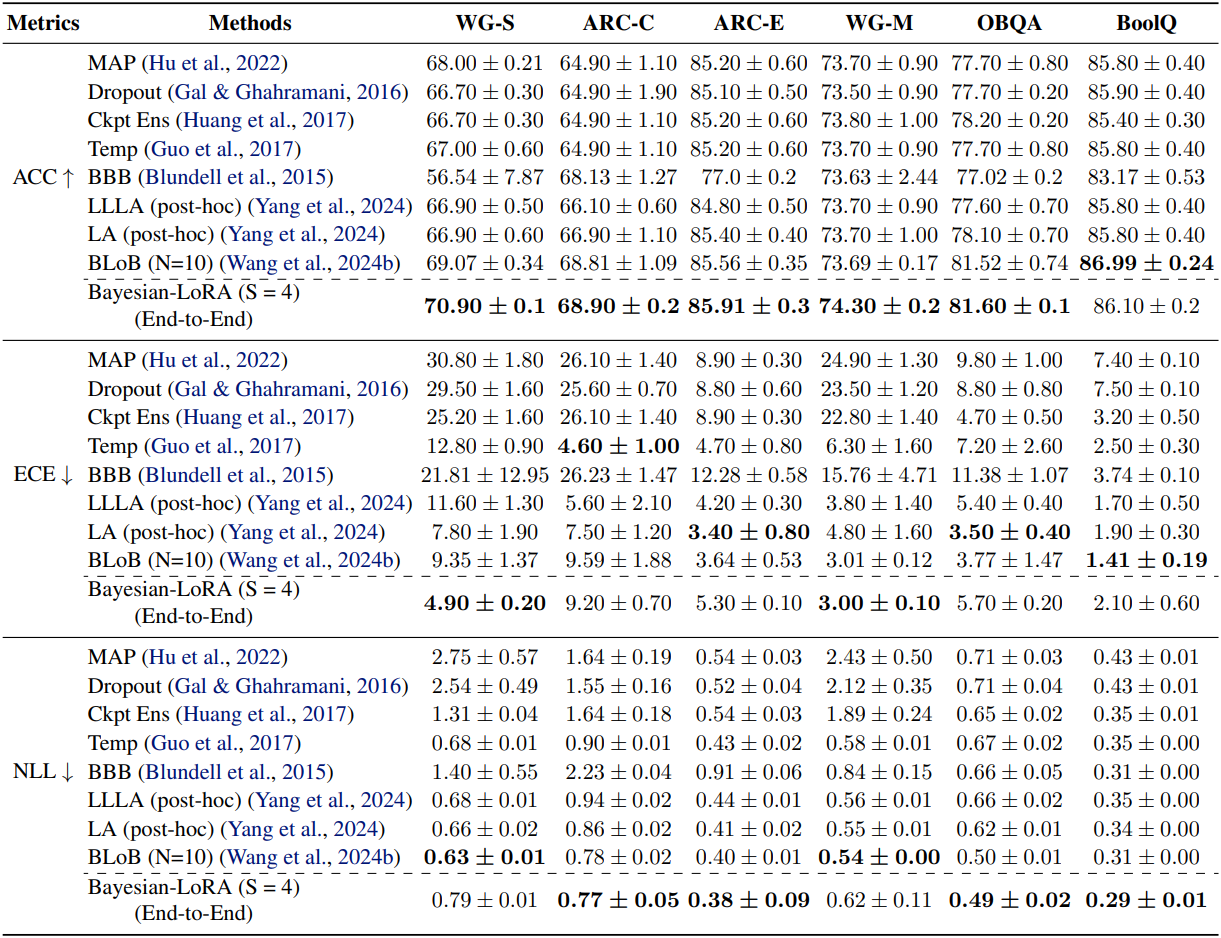
다음은 6가지 일반 상식 추론 벤치마크에 대한 비교 결과이다.

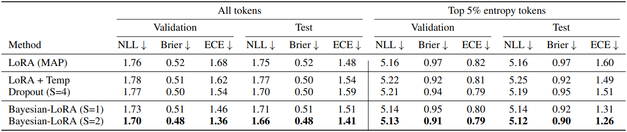
다음은 언어 모델링 성능을 비교한 결과이다. (WikiText-2)

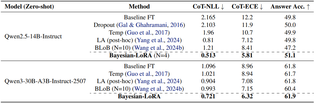
2. Scaling to Larger Architectures

다음은 대규모 모델에 대한 MATH 데이터셋 성능을 비교한 결과이다.

3. Efficiency Analysis

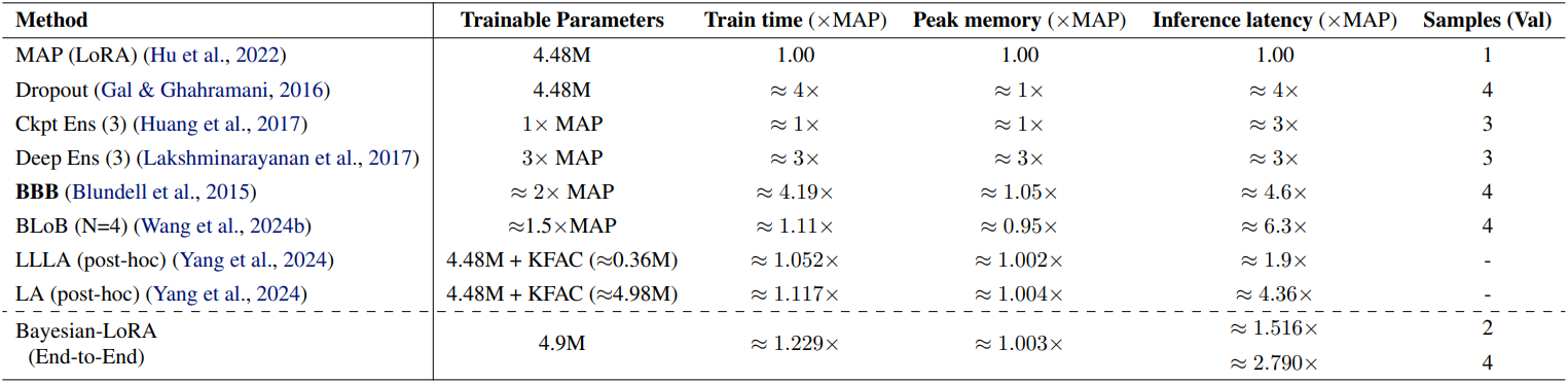
다음은 WinoGrande-M에서의 효율성 비교 결과이다.

4. Ablation Study

다음은 \(T_\phi\)의 flow depth $L$에 대한 ablation 결과이다.

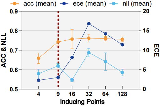
다음은 $U$의 차원 $r = c$에 대한 ablation 결과이다.

5. Out-of-Distribution Robustness

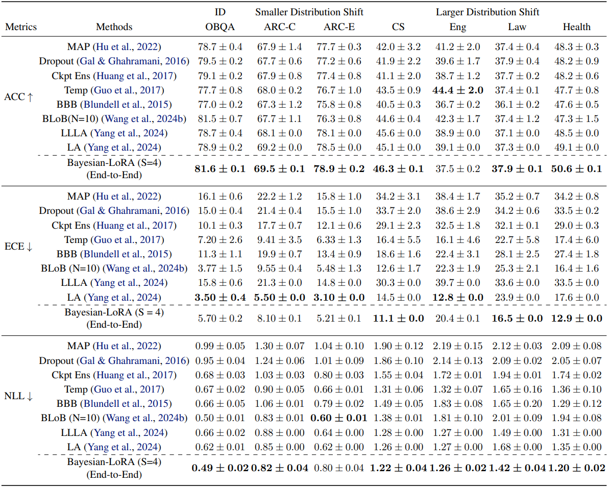
다음은 out-of-distribution에 대한 성능 비교 결과이다.