[논문리뷰] TRACT: Denoising Diffusion Models with Transitive Closure Time-Distillation

arXiv 2023. [Paper]
David Berthelot, Arnaud Autef, Jierui Lin, Dian Ang Yap, Shuangfei Zhai, Siyuan Hu, Daniel Zheng, Walter Talbott, Eric Gu
Apple
7 Mar 2023

Introduction

Diffusion model은 많은 도메인과 애플리케이션을 위한 state-of-the-art 생성 모델이다. Diffusion model은 주어진 데이터 분포의 score를 추정하는 방법을 학습하여 작동하며 실제로는 noise schedule에 따라 denoising autoencoder로 구현할 수 있다. Diffusion model을 학습시키는 것은 GAN, normalizing flow, autoregressive model과 같은 많은 생성 모델링 접근 방식에 비해 틀림없이 훨씬 간단하다. Loss가 명확하고 안정적이며, 아키텍처를 설계하는 데 상당한 유연성이 있고, discretization 필요 없이 연속적인 입력으로 직접 작동한다. 이러한 속성은 최근 연구에서 볼 수 있듯이 diffusion model이 대규모 모델 및 데이터셋에 대한 탁월한 확장성을 보여준다.

경험적 성공에도 불구하고 inference 효율성은 diffusion model의 주요 과제로 남아 있다. Diffusion model의 inference 프로세스는 discretization 오류가 감소함에 따라 샘플링 품질이 향상되는 neural ODE를 해결하는 것으로 캐스팅될 수 있다. 결과적으로 높은 샘플링 품질을 달성하기 위해 실제로 최대 수천 개의 denoising step이 사용된다. 많은 수의 inference step에 대한 이러한 의존성은 특히 리소스가 제한된 경우에서 GAN과 같은 one-shot 샘플링 방법에 비해 diffusion model을 불리하게 만든다.

Diffusion model의 inference 속도를 높이기 위한 기존 노력은 세 가지 클래스로 분류할 수 있다.

1. 입력 차원 줄이기
2. ODE solver 개선
3. 점진적인 distillation

이 중에서 점진적인 distillation 방식이 저자들의 관심을 불러일으켰다. DDIM inference schedule을 사용하면 초기 noise와 최종 생성된 결과 사이에 deterministic한 매핑이 있다는 사실을 이용한다. 이를 통해 주어진 teacher model에 근접한 효율적인 student model을 학습할 수 있다. 이러한 distillation의 naive한 구현은 각 student network 업데이트에 대해 teacher network를 $T$번 ($T$가 일반적으로 큰 경우) 호출해야 하기 때문에 금지된다. Progressive distillation에서는 Progressive Binary Time Distillation (BTD)를 수행하여 이 문제를 우회한다. BTD에서 distillation은 $\log_2 (T)$ phase로 나뉘고, 각 phase에서 student model은 두 개의 연속된 teacher model의 inference 결과를 학습한다. 실험적으로 BTD는 CIFAR-10과 64$\times$64 ImageNet에서 약간의 성능 손실로 inference step을 4개로 줄일 수 있다.

본 논문에서는 diffusion model의 inference 효율성을 극한으로 끌어올리는 것을 목표로 한다. 즉, 고품질 샘플을 사용한 one-step inference를 목표로 한다. 먼저 이 목표를 달성하지 못하게 하는 BTD의 중요한 단점을 식별한다.

1. 근사 오차가 한 distillation phase에서 다음 phase로 누적되어 목적 함수가 퇴보한다.
2. 학습 과정이 $\log_2 (T)$개의 phase로 구분되므로 우수한 일반화를 달성하기 위해 공격적인 stochastic weights averaging (SWA)를 사용하는 것을 방지한다.

이러한 관찰에 동기를 부여하여 TRAnsitive Closure Time-Distillation (TRACT)라는 새로운 diffusion model distillation 방식을 제안한다. 간단히 말해서, TRACT는 student model을 학습시켜 $t’ < t$인 step $t$에서 step $t’$까지의 teacher model의 inference 출력을 추출한다. $t \rightarrow t - 1$을 얻기 위해 teacher model의 한 step inference 업데이트를 수행한 다음 bootstrapping 방식으로 $t - 1 \rightarrow t’$을 얻기 위해 student model을 호출하여 목적 함수를 계산한다. Distillation이 끝나면 $t = T$와 $t’ = 0$으로 설정하여 teacher model로 one-step inference를 수행할 수 있다. 저자들은 TRACT가 한 phase 또는 두 phase로만 학습될 수 있음을 보여 BTD의 목적 함수 퇴보와 SWA 비호환성을 피한다.

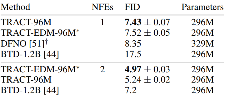
저자들은 실험적으로 TRACT가 one-step과 two-step의 inference로 state-of-the-art 결과를 크게 향상시킨다는 것을 확인하였다. 특히 64$\times$64 ImageNet와 CIFAR10에 대해 각각 7.4와 3.8의 one-step FID 점수를 달성했다.

Background

DDIM

(자세한 내용은 DDIM 논문 리뷰 참고)

DDIM은 $T$-step noise schedule $\gamma_t \in [0, 1)$을 사용하며, $t = 0$은 noise가 없는 step으로 $\gamma_0 = 1$이다. Variance preserving (VP) 세팅에서는 noisy한 샘플 $x_t$가 원본 샘플 $x_0$와 Gaussian noise $\epsilon$으로 생성된다.

\[\begin{equation} x_t = x_0 \sqrt{\gamma_t} + \epsilon \sqrt{1 - \gamma_t} \end{equation}\]

신경망 $f_\theta$는 신호나 noise, 또는 둘 모두를 예측하도록 학습된다. 각 step $t$의 $x_0$와 $\epsilon$의 추정값은 $x_{0 \vert t}$와 $\epsilon_{\vert t}$로 표현한다. 간결함을 위해 신호 예측 케이스만 설명한다. Denoisification phase에서 다음 식으로 예측된 $x_{0 \vert t}$를 사용하여 $\epsilon_{\vert t}$를 추정한다.

\[\begin{equation} x_{0 \vert t} := f_\theta (x_t, t), \quad \epsilon_{\vert t} = \frac{x_t - x_{0 \vert t} \sqrt{\gamma_t}}{\sqrt{1 - \gamma_t}} \end{equation}\]

이 추정으로 inference가 가능하다.

\[\begin{aligned} x_{t'} &= \delta (f_\theta, x_t, t, t') \\ & := x_t \frac{\sqrt{1 - \gamma_{t'}}}{\sqrt{1 - \gamma_t}} + f_\theta (x_t, t) \frac{\sqrt{\gamma_{t'} (1-\gamma_t)} - \sqrt{\gamma_t (1 - \gamma_{t'})}}{\sqrt{1 - \gamma_t}} \end{aligned}\]

여기서 step function $\delta$는 $x_t$에서 $x_{t’}$으로의 DDIM inference이다.

Binary Time-Distillation (BTD)

Student network $g_\phi$는 teacher $f_\theta$의 denoising step 2개를 교체하도록 학습된다.

\[\begin{equation} \delta (g_\phi, x_t, t, t-2) \approx x_{t-2} := \delta (f_\theta, \delta (f_\theta, x_t, t, t-1), t-1, t-2) \end{equation}\]

이 정의에 따라 위 방정식을 만족하는 target $\hat{x}$를 구할 수 있다.

\[\begin{equation} \hat{x} = \frac{x_{t-2} \sqrt{1 - \gamma_t} - x_t \sqrt{1 - \gamma_{t-2}}}{\sqrt{\gamma_{t-2}} \sqrt{1 - \gamma_t} - \sqrt{\gamma_t} \sqrt{1 - \gamma_{t-2}}} \end{equation}\]

다음과 같은 noise 예측 오차로 loss를 다시 쓸 수 있다.

\[\begin{equation} \mathcal{L} (\phi) = \frac{\gamma_t}{1 - \gamma_t} \| g_\phi (x_t, t) - \hat{x} \|_2^2 \end{equation}\]

Student가 완료될 때까지 학습하면 teacher가 되며 최종 모델이 원하는 step 수를 가질 때까지 프로세스가 반복된다. $T$-step teacher를 one-step 모델로 distillation하는 데 $\log_2 T$개의 학습 phase가 필요하며, 학습된 각 student는 고품질 샘플을 생성하기 위해 teacher의 샘플링 step의 절반이 필요하다.

Method

본 논문은 distillation phase의 수를 $\log_2 T$에서 작은 상수(일반적으로 1 또는 2)로 줄이는 BTD의 확장인 TRAnsitive Closure Time-Distillation (TRACT)를 제안합다. 먼저 BTD에서 사용되는 VP 세팅에 중점을 두지만 방법은 그 자체는 그것과 독립적이며 Variance Exploding(VE) 세팅에서 사용 가능하다. TRACT는 noise 예측 목적함수에도 작동하지만 신경망이 $x_0$의 추정치를 예측하는 신호 예측에서 작동한다.

1. Motivation

저자들은 distill된 모델에서 샘플의 최종 품질이 distillation phase의 수와 각 phase의 길이에 의해 영향을 받는다고 추측하였다. 왜 그런지에 대한 두 가지 잠재적인 설명을 고려한다.

Objective degeneracy

BTD에서는 이전 distillation phase의 student가 다음 phase의 teacher가 된다. 이전 phase의 student는 다음 phase에서 불완전한 teacher를 낳는 positive loss를 가지고 있다. 이러한 불완전성은 teacher들의 연속적인 세대에 걸쳐 축적되어 목적 함수의 퇴보로 이어진다.

Generalization

Stochastic Weight Averaging (SWA)은 DDPM용으로 학습된 신경망의 성능을 개선하는 데 사용되었다. Exponential Moving Average (EMA)를 사용하면 모멘텀 파라미터가 학습 길이에 의해 제한된다. 높은 모멘텀은 고품질 결과를 산출하지만 학습 길이가 너무 짧으면 과도하게 정규화된 모델로 이어진다. 이것은 총 학습 길이가 학습 phase의 수에 정비례하기 때문에 시간 distillation 문제와 관련이 있다.

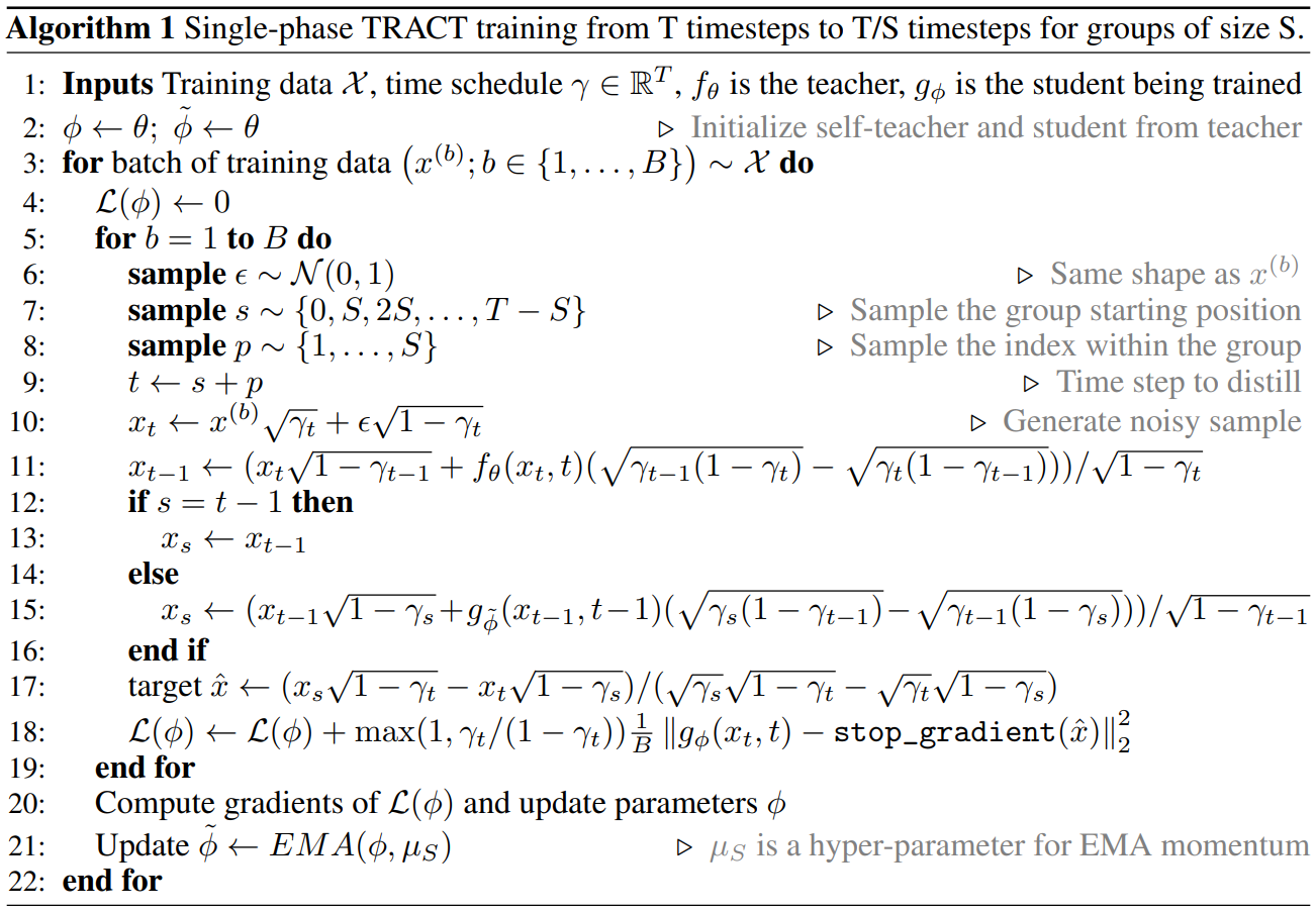
2. TRACT

TRACT는 각 phase가 $T$-step schedule을 $T’ < T$ step으로 증류하고 원하는 step 수에 도달할 때까지 반복되는 multi-phase 방법이다. 한 phase에서 $T$-step schedule은 $T’$개의 연속 그룹으로 분할된다. 분할 전략은 어떤 것도 사용할 수 있다. 예를 들어 실험에서는 Algorithm 1과 같이 동일한 크기의 그룹을 사용했다.

본 논문의 방법은 $T’ = T/2$에 의해 제한되지 않는 BTD의 확장으로 볼 수 있다. 그러나 $t’ < t$에 대해 $x_t$에서 $x_t’$을 추정하는 것과 같이 이 제약 조건의 완화로 인해 계산상의 의미가 생긴다.

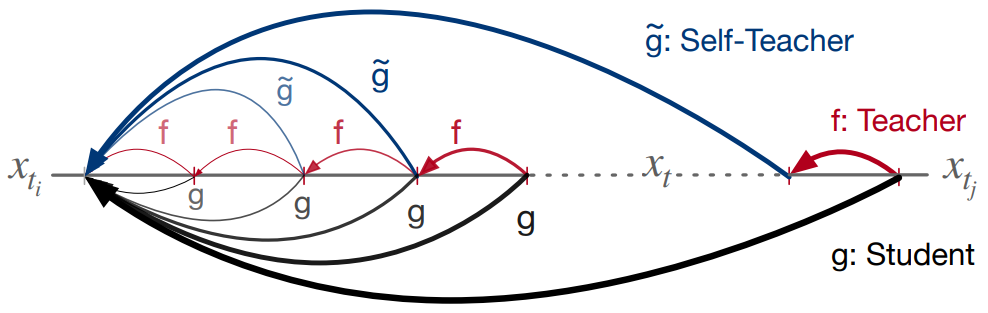
연속 세그먼트 \(\{t_i, \cdots, t_j\}\)에 대하여, 위 그림과 같이 student $g_\phi$가 임의의 step $t_i < t \le t_j$에서 step $t_i$로 점프하도록 모델링한다.

\[\begin{equation} \delta (g_\phi, x_t, t, t_i) = \delta (f_\theta, \delta (f_\theta, \cdots, \delta (f_\theta, x_t, t, t-1), \cdots), t_{i+1}, t_i) \end{equation}\]

Student $g$는 $f$의 denoising step $(t_j - t_i)$를 포함하도록 지정된다. 그러나 이 공식은 학습 중에 $f$를 여러 번 호출해야 하므로 엄청난 계산 비용이 발생할 수 있다.

이 문제를 해결하기 위해 가중치가 student $g$의 EMA인 self-teacher를 사용한다. 이 접근 방식은 semi-supervised learning, 강화 학습, 표현 학습에서 영감을 받았다. 가중치가 $\phi$인 student network $g$의 경우 가중치의 EMA를 $\tilde{\phi} = \textrm{EMA} (\phi, \mu_S)$로 표시한다. 여기서 모멘텀인 $\mu_S \in [0, 1]$는 hyper-parameter이다.

따라서 transitive closure operator는 위 방정식을 다시 써서 self-teaching으로 모델링할 수 있다.

\[\begin{equation} \delta (g_\phi, x_t, t, t_i) \approx x_{t_i} := \delta (g_{\tilde{\phi}}, \delta (f_\theta, x_t, t, t-1), t-1, t_i) \end{equation}\]

이 정의로부터 방정식을 만족하는 target $\hat{x}$를 결정할 수 있다.

\[\begin{equation} \hat{x} = \frac{x_{t_i} \sqrt{1 - \gamma_t} - x_t \sqrt{1 - \gamma_{t_i}}}{\sqrt{\gamma_{t_i}} \sqrt{1 - \gamma_t} - \sqrt{\gamma_t} \sqrt{1 - \gamma_{t_i}}} \end{equation}\]

$t_i = t-1$인 경우 $\hat{x} = f_\theta (x_t, t)$가 된다.

$\hat{x}$에 대한 loss는 다음과 같다.

\[\begin{equation} \mathcal{L} (\phi) = \frac{\gamma_t}{1 - \gamma_t} \| g_\phi (x_t, t) - \hat{x} \|_2^2 \end{equation}\]

3. Adapting TRACT to a Runge-Kutta teacher and Variance Exploding noise schedule

일반성을 설명하기 위해 VE noise schedule과 RK sampler를 사용하는 Elucidating the Design space of diffusion Model (EDM)의 teacher에게 TRACT를 적용한다.

VE noise schedules

VE noise schedule은 \(\sigma_1 = \sigma_{min} \le \sigma_t \le \sigma_T = \sigma_{max}\)인 \(t \in \{1, \cdots, T\}\)에 대한 일련의 noise 표준 편차 $\sigma_t \ge 0$으로 parameterize되고 $t = 0$은 noise가 없는 step $\sigma_0 = 0$을 나타낸다. 다음과 같이 원본 샘플 $x_0$와 Gaussian noise $\epsilon$에서 noisy한 샘플 $x_t$가 생성된다.

\[\begin{equation} x_t = x_0 + \sigma_t \epsilon \end{equation}\]

RK step function

EDM 접근 방식에 따라 teacher로 RK sampler를 사용하고 student로 DDIM sampler를 distill한다. Step function은 각각 $\delta_{RK}$와 $\delta_{DDIM-VE}$이다. $x_t$에서 $x_t’$을 추정하는 $\delta_{RK}$ step function ($t > 0$)은 다음과 같이 정의된다.

\[\begin{equation} \delta_{RK} (f_\theta, x_t, t, t') := \begin{cases} x_t + (\sigma_{t'} - \sigma_t) \epsilon (x_t, t) & \textrm{if } t' = 0 \\ x_t + \frac{1}{2} (\sigma_{t'} - \sigma_t) [\epsilon (x_t, t) + \epsilon (x_t + (\sigma_{t'} - \sigma_t) \epsilon (x_t, t), t)] & \textrm{otherwise} \end{cases} \\ \textrm{where} \quad \epsilon (x_t, t) := \frac{x_t - f_\theta (x_t, t)}{\sigma_t} \end{equation}\]

$x_t$에서 $x_{t’}$을 추정하는 $\delta_{DDIM-VE}$ step function은 다음과 같이 정의된다.

\[\begin{equation} \delta_{DDIM-VE} (f_\theta, x_t, t, t') := f_\theta (x_t, t) \bigg( 1 - \frac{\sigma_{t'}}{\sigma_t} \bigg) + \frac{\sigma_{t'}}{\sigma_t} x_t \end{equation}\]

그러면 self-teaching을 통해 transitive closure operator를 학습하려면 다음 식이 필요하다.

\[\begin{equation} \delta_{DDIM-VE} (f_\theta, x_t, t, t') \approx x_{t_i} := \delta_{DDIM-VE} (g_{\tilde{\phi}}, \delta_{RK} (f_\theta, x_t, t, t-1), t-1, t_i) \end{equation}\]

이 정의로부터 방정식을 만족하는 target $\hat{x}$를 결정할 수 있다.

\[\begin{equation} \hat{x} = \frac{\sigma_t x_{t_i} - \sigma_{t_i} x_t}{\sigma_t - \sigma_{t'}} \end{equation}\]

그러면 Loss는 student network의 예측과 $\hat{x}$ 사이의 가중된 loss가 된다.

\[\begin{equation} \mathcal{L}(\phi) = \lambda (\sigma_t) \| g_\phi (x_t, t) - \hat{x} \|_2^2 \end{equation}\]

Experiment

1. Image generation results

CIFAR-10

다음은 CIFAR-10에서의 FID 결과를 나타낸 표이다.

   

64$\times$64 ImageNet

다음은 64$\times$64 ImageNet에서의 FID 결과를 나타낸 표이다.

   

2. Stochastic Weight Averaging ablations

저자들은 실험에서 bias-corrected EMA를 사용하였다.

\[\begin{aligned} \tilde{\phi}_0 &= \phi_0 \\ \tilde{\phi}_i &= \bigg(1 - \frac{1 - \mu_S}{1 - \mu_S^i} \bigg) \tilde{\phi}_{i-1} + \frac{1 - \mu_S}{1 - \mu_S^i} \phi_i \end{aligned}\]

Ablation study에서 distillation schedule은 $1024 \rightarrow 32 \rightarrow 1$로 고정하였으며, phase당 4800만 개의 샘플을 사용하였다.

Self-teaching EMA

다음은 $\mu_I = 0.99995$로 고정하고 $\mu_S$에 대한 ablation study를 진행한 결과이다. (CIFAR-10)

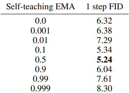
$\mu_S$의 값이 넓은 범위에서 좋은 성능을 보인다는 것을 확인할 수 있다.

Inference EMA

$\mu_S = 0.5$로 고정하고 $\mu_I$에 대한 ablation study를 진행한 결과이다. (CIFAR-10)

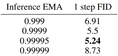
$\mu_I$의 값이 성능에 큰 영향을 준다는 것을 확인할 수 있다.

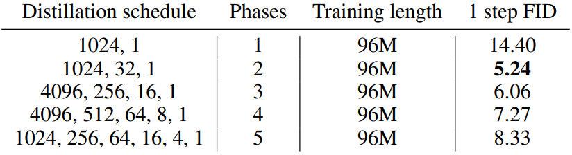
3. Influence of the number of distillation phases

Fixed overall training length

다음은 전체 학습 길이를 고정하였을 때의 ablation 결과이다.

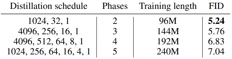
Fixed training length per phase

다음은 phase당 학습 길이를 고정하였을 때의 ablation 결과이다.

Binary Distillation comparison

저자들은 목적 함수 퇴보가 TRACT가 BTD를 능가하는 이유임을 추가로 확인하기 위해 동일한 BTD에 호환되는 schedule ($1024 \rightarrow 512 \rightarrow \cdots \rightarrow 2 \rightarrow 1$)에서 BTD를 TRACT과 비교하였다. 두 실험 모두 $\mu_I = 0.99995$로 설정하고 phase당 4800만개의 샘플을 사용하였다. 이 설정에서 BTD의 FID는 5.95, TRACT의 FID는 6.8이며, BTD는 TRACT를 능가한다. 이는 BTD의 열악한 전체 성능이 2-phase schedule을 활용할 수 없기 때문일 수 있음을 추가로 확인한다.

Schedule 외에도 BTD와 TRACT의 차이점은 TRACT의 self-teaching의 사용이다. 이 실험은 또한 self-teaching 교육이 supervised 학습보다 덜 효율적인 목적 함수를 초래할 수 있음을 시사한다.