[논문리뷰] PriorGrad: Improving Conditional Denoising Diffusion Models with Data-Driven Adaptive Prior
ICLR 2022. [Paper] [Page]
Sang-gil Lee, Heeseung Kim, Chaehun Shin, Xu Tan, Chang Liu, Qi Meng, Tao Qin, Wei Chen, Sungroh Yoon, Tie-Yan Liu
Data Science & AI Lab., Seoul National University | Microsoft Research Asia
11 Jun 2021
Introduction
Diffusion 기반 음성 합성 모델은 고품질 음성 오디오 생성을 달성했지만 잠재적인 비효율성을 나타내므로 고급 전략이 필요할 수 있다. 예를 들어, 모델은 학습 중에 상당히 느린 수렴으로 어려움을 겪고 있으며 대략적인 reverse process를 학습하는 데 엄청난 학습 계산 시간이 필요하다. 기존의 diffusion 기반 모델은 표준 Gaussian을 사전 분포로 정의하고 신호를 prior noise로 절차적으로 파괴하는 non-parametric diffusion process를 설계한다. 심층 신경망은 데이터 밀도의 기울기를 추정하여 reverse process를 근사화하도록 학습된다. 표준 Gaussian을 prior에 적용하는 것은 대상 데이터에 대한 가정 없이 간단하지만 비효율적이다. 예를 들어, 시간 도메인 waveform 데이터에서 신호는 음성이 있는 부분과 음성이 없는 부분과 같은 서로 다른 세그먼트 간에 매우 높은 가변성을 갖는다. 동일한 표준 Gaussian prior으로 유성음 및 무성음 세그먼트를 공동으로 모델링하는 것은 모델이 데이터의 모든 mode를 다루기 어려울 수 있으므로 학습 비효율과 잠재적으로 잘못된 diffusion 궤적을 초래할 수 있다.
이전 추론을 바탕으로 다음 질문을 평가한다.
조건부 diffusion 기반 모델의 경우 추가 계산 또는 파라미터 복잡성을 통합하지 않고 보다 유익한 prior를 공식화할 수 있는가?
이를 조사하기 위해 본 논문은 조건 정보를 기반으로 forward process에 대한 평균과 분산을 직접 계산하여 적응 noise를 사용하는 PriorGrad라는 간단하면서도 효과적인 방법을 제안한다. 구체적으로 조건부 음성 합성 모델을 사용하여 vocoder에 대한 mel-spectrogram과 acoustic model에 대한 음소와 같은 조건부 데이터를 기반으로 prior 분포를 구조화할 것을 제안한다. 프레임 수준(vocoder) 또는 음소 수준(acoustic model) 세분성에서 조건부 데이터의 통계를 계산하고 Gaussian prior의 평균 및 분산으로 매핑하여 대상 데이터 분포와 유사한 noise를 구조화할 수 있으며, 인스턴스 레벨에서 reverse process를 배우는 부담을 덜어준다.
Background
Forward process:
\[\begin{aligned} q(x_{1:T} \vert x_0) &= \prod_{t=1}^T q(x_t \vert x_{t-1}) \\ q(x_t \vert x_{t-1}) &:= \mathcal{N} (x_t; \sqrt{1 - \beta_t} x_{t-1}, \beta_t I) \end{aligned}\] \[\begin{equation} q(x_t \vert x_0) = \mathcal{N}(x_t; \sqrt{\vphantom{1} \bar{\alpha}_t} x_0, (1 - \bar{\alpha}_t) I) \\ \alpha_t := 1 - \beta_t, \quad \bar{\alpha}_t := \prod_{s=1}^t \alpha_s \end{equation}\]Reverse process:
\[\begin{aligned} p_\theta (x_{0:T}) &= p(x_T) \prod_{t=1}^T p_\theta (x_{t-1} \vert x_t) \\ p_\theta (x_{t-1} \vert x_t) &= \mathcal{N} (x_{t-1}; \mu_\theta (x_t, t), \Sigma_\theta (x_t, t)) \end{aligned}\]목적 함수:
\[\begin{aligned} L(\theta) &= \mathbb{E}_q \bigg[ \textrm{KL} (q(x_T \vert x_0) \;\|\; p(x_T)) \\ &\quad\quad + \sum_{t=2}^T \textrm{KL} (q(x_{t-1} \vert x_t, x_0) \;\|\; p_\theta (x_{t-1} \vert x_t)) \\ &\quad\quad - \log p_\theta (x_0 \vert x_1) \bigg] \end{aligned}\] \[\begin{equation} q(x_{t-1} \vert x_t, x_0) = \mathcal{N} (x_{t-1}; \tilde{\mu}(x_t, x_0), \tilde{\beta}_t I) \\ \tilde{\mu}_t (x_t, x_0) := \frac{\sqrt{\vphantom{1} \bar{\alpha}_{t-1}} \beta_t}{1 - \bar{\alpha}_t} x_0 + \frac{\sqrt{\alpha_t} (1 - \bar{\alpha}_{t-1})}{1 - \bar{\alpha}_t} x_t \\ \tilde{\beta}_t := \frac{1 - \bar{\alpha}_{t-1}}{1 - \bar{\alpha}_t} \beta_t \end{equation}\]ELBO:
\[\begin{equation} -\textrm{ELBO} = C + \sum_{t=1}^T \mathbb{E}_{x_0, \epsilon} [ \gamma_t \| \epsilon - \epsilon_\theta (\sqrt{\vphantom{1} \bar{\alpha}_t} x_0 + \sqrt{1 - \bar{\alpha}_t} \epsilon , t) \|^2 ] \\ \gamma_t = \frac{\beta_t^2}{2 \sigma_t^2 \alpha_t (1 - \bar{\alpha}_t)} \end{equation}\]단순화된 목적 함수:
\[\begin{equation} L_\textrm{simple} (\theta) := \mathbb{E}_{t, x_0, \epsilon}[\| \epsilon - \epsilon_\theta (x_t, t) \|^2] \end{equation}\]Method
1. General Formulation
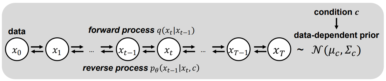
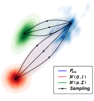
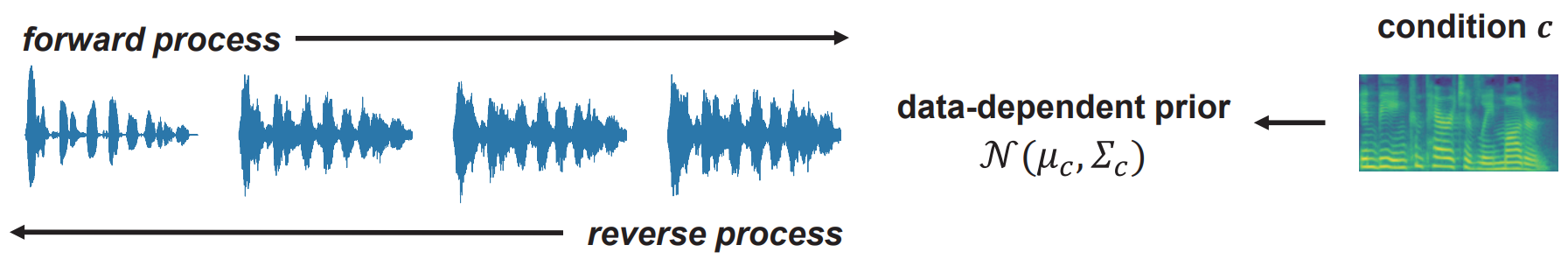
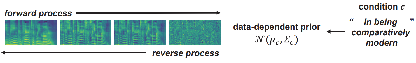
표준 Gaussian이 아닌 $\mathcal{N}(\mu, \Sigma)$를 forward diffusion prior로 사용하는 방법의 일반적인 공식을 다룬다. PriorGrad는 조건부 데이터를 활용하여 적응 방식으로 인스턴스 레벨 근사 prior를 직접 계산하고 학습 및 inference 모두에 대한 forwad diffusion 대상으로 근사 prior을 사용한다. 위 그림들은 시각적으로 높은 레벨의 개요를 보여준다. 원래 DDPM에서와 동일한 $\mu_\theta$와 $\sigma_\theta$의 parameterization을 사용한다.
Forward diffusion의 사전 분포로 최적의 Gaussian $\mathcal{N}(\mu, \Sigma)$에 액세스할 수 있다고 가정하면 다음과 같은 수정된 ELBO를 따른다.
\[\begin{equation} -\textrm{ELBO} = C(\Sigma) + \sum_{t=1}^T \gamma_t \mathbb{E}_{x_0, \epsilon} \| \epsilon - \epsilon_\theta (\sqrt{\vphantom{1} \bar{\alpha}_t} (x_0 - \mu) + \sqrt{1 - \bar{\alpha}_t} \epsilon , t) \|_{\Sigma^{-1}}^2 \end{equation}\]여기서 \(\| x \|_{\Sigma^{-1}}^2 = x^\top \Sigma x\)이다.
데이터에 대한 가정 없이 $\mathcal{N} (0, I)$을 prior로 사용했던 기존 DDPM과 달리 데이터에서 평균과 분산을 추출한 $\mathcal{N} (\mu, \Sigma)$를 forward process를 위한 prior로 사용한다.
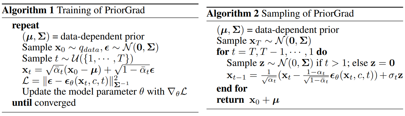
또한 이전 연구를 따라 학습을 위한 단순화된 loss
\[\begin{equation} \mathcal{L} = \| \epsilon - \epsilon_\theta (x_t, c, t) \|_{\Sigma^{-1}}^2 \end{equation}\]로 $\gamma_t$를 삭제한다. Algorithm 1과 2는 데이터 종속 prior $(\mu, \Sigma)$에 의해 강화된 학습 및 샘플링 절차를 설명한다. 데이터 종속 prior 계산은 애플리케이션에 종속이므로 주어진 task에 대한 조건부 데이터를 기반으로 이러한 prior 계산을 설명한다.
2. Theoretical Analysis
Simplified modeling
Proposition
$L(\mu, \Sigma, x_0; \theta)$를 수정된 $-\textrm{ELBO}$ loss라 하고, $\epsilon_\theta$가 선형 함수라 가정하자. $\textrm{det}(\Sigma) = \textrm{det}(I)$라는 제약 하에서
\[\begin{equation} \min_\theta L(\mu, \Sigma, x_0; \theta) \le \min_\theta L(0,I,x_0; \theta) \end{equation}\]이다.
위의 Proposition은 공분산 $\Sigma$가 데이터 $x_0$의 공분산과 일치하는 prior 설정이 $theta$에 대한 선형 함수 근사를 사용하는 경우 loss가 더 적다는 것을 보여준다. 이는 데이터 종속 prior에서 $q(x_{t-1} \vert x_t)$의 평균을 나타내기 위해 간단한 모델을 사용할 수 있는 반면, 등방성 공분산이 있는 prior에서 동일한 정밀도를 달성하려면 복잡한 모델을 사용해야 함을 나타낸다. 조건 $\textrm{det}(\Sigma) = \textrm{det}(I)$는 두 개의 Gaussian prior 값이 동일한 엔트로피를 갖는다는 것을 의미하며, 이는 공정한 비교를 위한 조건이다.
Convergence rate
최적화의 수렴율은 loss function $H$의 Hessian 행렬의 condition number, 즉 \(\lambda_\textrm{max} (H) / \lambda_\textrm{min} (H)\)에 따라 달라지며, 여기서 \(\lambda_\textrm{max}\)와 \(\lambda_\textrm{min}\)은 각각 $H$의 고유값의 최대값과 최소값이다. Condition number가 작을수록 수렴 속도가 빨라진다. $L(\mu, \Sigma, x_0; \theta)$의 경우 Hessian은 다음과 같이 계산된다.
\[\begin{equation} H = \frac{\partial^2 L}{\partial \epsilon_\theta^2} \cdot \frac{\partial \epsilon_\theta}{\partial \theta} \cdot \bigg( \frac{\partial \epsilon_\theta}{\partial \theta} \bigg)^\top + \frac{\partial L}{\partial \epsilon_\theta} \cdot \frac{\partial^2 \epsilon_\theta}{\partial \theta^2} \end{equation}\]$\epsilon_\theta$가 선형 함수라고 가정한다면, $L(\mu, \Sigma, x_0; \theta)$의 경우 $H \propto I$이고 $L(0,I,x_0; theta)$의 경우 $H \propto \Sigma + I$이다. Prior을 $\mathcal{N} (\mu, \Sigma)$로 설정하면 $H$의 condition number가 1이 되어 condition number가 가장 작은 값이 되는 것이 분명하다. 따라서 수렴을 가속화할 수 있다.
Application to Vocoder
1. PriorGrad for Vocoder
Vocoder에 적용되는 PriorGrad는 DiffWave를 기반으로 한다. 여기서 모델은 데이터의 컴팩트한 주파수 feature 표현을 포함하는 mel-spectrogram을 조건으로 하는 시간 도메인 waveform을 합성한다. $\epsilon \sim \mathcal{N}(0, I)$를 사용한 이전 방법과 달리, PriorGrad 네트워크는 파괴된 신호 \(\bar{\alpha}_t x_0 + \sqrt{1 - \bar{\alpha}_t} \epsilon\)가 주어지면 noise $\epsilon \sim \mathcal{N} (0, \Sigma)$를 추정하도록 학습된다. 네트워크는 또한 diffusion-step embedding layer가 있는 noise level $\sqrt{\vphantom{1} \bar{\alpha}_t}$의 discretize된 인덱스와 조건부 projection layer가 있는 mel-spectrogram $c$로 컨디셔닝된다.
Mel-spectrogram 조건을 기반으로 스펙트럼 에너지가 waveform 분산에 대한 정확한 상관관계를 포함한다는 사실을 이용하여 데이터 종속 prior를 얻기 위해 mel-spectrogram의 정규화된 프레임 레벨 에너지를 활용한다. 먼저 학습 데이터셋의 mel-spectrogram $c$에 지수의 합의 제곱근을 적용하여 프레임 레벨 에너지를 계산한다. 그런 다음 프레임 레벨 에너지를 $(0, 1]$ 범위로 정규화하여 데이터 종속 대각 분산 $\Sigma_c$를 얻는다. 이러한 방식으로 프레임 레벨 에너지를 waveform 데이터에 대한 표준 편차로 사용할 수 있다. 이것은 mel-scale spectral energy와 diagonal Gaussian의 표준 편차 사이의 비선형 매핑으로 간주될 수 있다.
주어진 vocoder에 대한 hop length를 사용하여 프레임 레벨의 $\Sigma_c$를 waveform 레벨의 $\Sigma$로 업샘플링하여 각 학습 step에 대한 forward diffusion prior로 $\mathcal{N}(0, \Sigma)$를 설정한다. Waveform 분포의 평균이 0이라는 사실을 반영하여 prior의 평균을 0으로 선택한다. 실제로는 학습 중 수치적 안정성을 보장하기 위해 클리핑을 통해 prior의 최소 표준편차를 0.1로 부과한다. Prior를 계산하기 위해 음성이 있거나 없는 레이블 및 음소 레벨 통계와 같은 조건부 정보의 여러 대체 소스를 시도했지만 결과적으로 성능이 저하된다고 한다.
2. Experiments Results
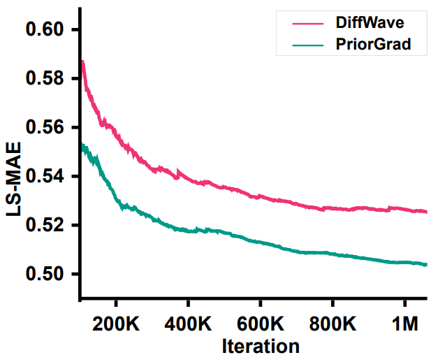
다음은 vocoder 모델의 수렴 결과를 LS-MAE (log-mel spectrogram mean absolute error)로 나타낸 그래프이다.
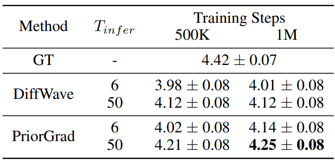
다음은 5점 MOS로 PriorGrad vocoder를 주관적으로 평가한 표이다.
다음은 다양한 객관적 지표를 나타낸 표이다. (100만 step 학습)

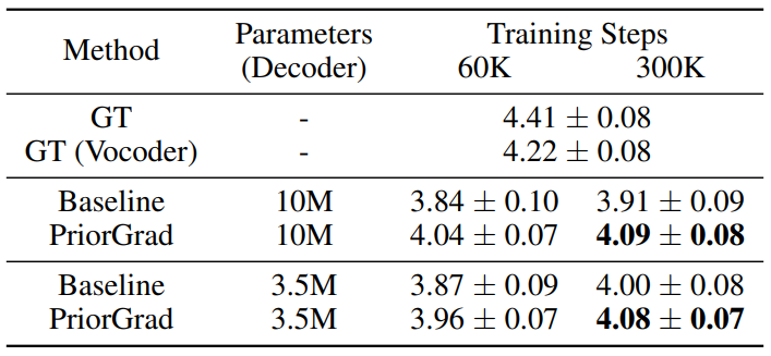
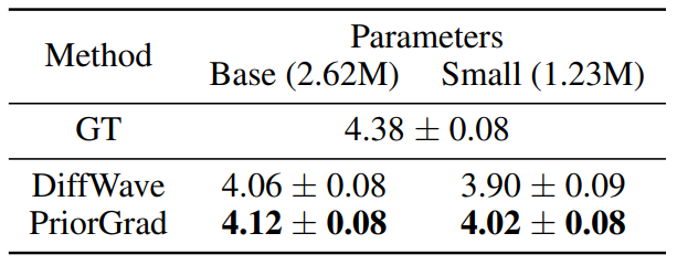
다음은 모델의 capacity를 줄였을 때의 MOS 결과를 나타낸 표이다. (100만 step 학습)
Application to Acoustic Model
1. PriorGrad for Acoustic Model
Acoustic model은 인코더 디코더 아키텍처를 사용하여 일련의 음소가 주어지면 mel-spectrogram을 생성한다. 즉, acoustic model은 타겟 이미지가 2D mel-spectrogram인 텍스트 조건부 이미지 생성 task와 유사하다. 본 논문은 Fastspeech 2의 접근 방식을 feed-forward 음소 인코더로 사용하고 Diffwave를 기반으로 dilated convolutional layer가 있는 diffusion 기반 디코더를 사용하여 PriorGrad acoustic model을 구현한다.
적응형 prior을 구축하기 위해 학습 데이터에서 동일한 음소에 해당하는 프레임을 집계하여 80-band mel-spectrogram 프레임의 음소 레벨 통계를 계산한다. 여기서 음소-프레임 alignment는 Montreal forced alignment (MFA) tookit을 사용한다. 구체적으로, 각 음소에 대해 학습 데이터셋의 모든 occurrence를 집계하여 80차원 대각 평균과 분산을 얻는다. 그런 다음 음소당 $\mathcal{N}(\mu, \Sigma)$ prior을 구성한다. Forward diffusion prior에 이러한 통계를 사용하려면 음소 레벨 prior 시퀀스를 일치하는 duration의 프레임 레벨로 업샘플링해야 한다. 이는 duration predictor 모듈을 기반으로 하는 음소 인코더 출력과 동일한 prior에 이 음소 레벨을 공동으로 업샘플링함으로써 수행될 수 있다.
Algorithm 1에 따라 평균이 이동한 noisy한 mel-spectrogram
\[\begin{equation} x_t = \sqrt{\vphantom{1} \bar{\alpha}_t} (x_0 - \mu) + \sqrt{1 - \bar{\alpha}_t} \epsilon \end{equation}\]을 입력으로 사용하여 diffusion 디코더 네트워크를 학습시킨다. 네트워크는 주입된 noise $\epsilon \sim \mathcal{N} (0, \Sigma)$를 타겟으로 추정한다. 네트워크는 추가로 align된 음소 인코더 출력으로 컨디셔닝된다. 인코더 출력은 계층별 1$\times$1 convolutional이 있는 gated residual block의 각 dilated convolution layer의 bias 항으로 추가된다.
2. Experiments Results
다음은 PriorGrad acoustic model의 MOS 결과이다. (95% 신뢰 구간)