[논문리뷰] On Distillation of Guided Diffusion Models
CVPR 2023. [Paper]
Chenlin Meng, Robin Rombach, Ruiqi Gao, Diederik P. Kingma, Stefano Ermon, Jonathan Ho, Tim Salimans
Stanford University | Stability AI & LMU Munich | Google Research, Brain Team
6 Oct 2022
Introduction
DDPM은 이미지 생성이나 오디오 합성 등 다양한 분야에서 state-of-the-art 성능을 달성했다. Classifier-free guidance는 diffusion model의 샘플 품질을 더욱 향상시키고 GLIDE, Stable Diffusion, DALL·E 2, Imagen을 포함한 대규모 diffusion model 프레임워크에서 널리 사용되었다. 그러나 classifier-free guidance의 주요 제한 사항 중 하나는 샘플링 효율성이 낮다는 것이다. 하나의 샘플을 생성하기 위해 두 diffusion model을 수십에서 수백 번 평가해야 한다. 이러한 제한은 실제 설정에서 classifier-free guidance model의 적용을 방해했다.
Diffusion model에 대해 distillation 접근법이 제안되었지만 이러한 접근법은 classifier-free guided diffusion model에 직접 적용할 수 없다. 본 논문은 classifier-free guided model의 샘플링 효율성을 개선하기 위한 2단계 distillation 방식을 제안한다. 첫 번째 stage에서는 teacher의 두 가지 diffusion model의 결합된 출력과 일치하도록 단일 student 모델을 도입한다. 두 번째 stage에서는 첫 번째 stage에서 학습한 모델을 더 적은 step의 모델로 점진적으로 distill한다. 본 논문의 접근 방식을 사용하면 단일 distillation model이 다양한 guidance 강도를 광범위하게 처리할 수 있으므로 샘플 품질과 다양성 간의 균형을 효율적으로 유지할 수 있다. 모델에서 샘플링하기 위해 기존 deterministic 샘플러를 고려하고 stochastic 샘플링 프로세스를 추가로 제안한다.
본 논문의 distillation 프레임워크는 pixel-space에서 학습된 표준 diffusion model뿐만 아니라 autoencoder의 latent-space에서 학습된 diffusion model(ex. Stable Diffusion)에도 적용될 수 있다. Pixel-space에서 직접 학습된 diffusion model의 경우 제안된 distillation model이 4 step만 사용하여 teacher model과 시각적으로 비슷한 샘플을 생성할 수 있고 비슷한 FID/IS 점수를 달성할 수 있다. 광범위한 guidance 강도에 대해 4~16 step을 사용하는 teacher model로 사용한다 (위 그림 참고). 인코더의 latent-space에서 학습된 diffusion model의 경우, 최소 1~4개의 샘플링 step을 사용하여 base model과 비슷한 시각적 품질을 달성할 수 있으며, 2~4개의 샘플링 step만으로 teacher의 성능과 일치한다. 본 논문은 pixel-space 및 latent-space classifier-free diffusion model에 대한 distillation의 효율성을 처음으로 입증하였다.
Background on diffusion models
데이터 분포 $p_\textrm{data} (x)$의 샘플 $x$와 noise schedule $\alpha_t$, $\sigma_t$가 주어지면 가중 MSE를 최소화하여 diffusion model \(\hat{x}_\theta\)를 학습시킨다.
\[\begin{equation} \mathbb{E}_{t \sim U[0, 1], x \sim p_\textrm{data} (x), z_t \sim q(z_t \vert x)} [w(\lambda_t) \| \hat{x}_\theta - x \|_2^2] \end{equation}\]여기서 $\lambda_t = \log [\alpha_t^2 / \sigma_t^2]$은 SNR(신호 대 잡음비)이고 $q(z_t \vert x) = \mathcal{N}(z_t; \alpha_t x, \sigma_t^2 I)$와 $w(\lambda_t)$는 미리 정의된다.
Diffusion model \(\hat{x}_\theta\)가 학습되면 discrete-time DDIM sampler를 사용하여 샘플링을 할 수 있다. 구체적으로 DDIM sampler는 $z_1 \sim \mathcal{N}(0,I)$에서 시작하여 다음과 같이 업데이트된다.
\[\begin{equation} z_s = \alpha_s \hat{x}_\theta (z_t) + \sigma_s \frac{z_t - \alpha_S \hat{x}_\theta (z_t)}{\sigma_t}, \quad s = t - \frac{1}{N} \end{equation}\]여기서 $N$은 전체 샘플링 step 수이다.
Classifier-free guidance
(자세한 내용은 논문 리뷰 참고)
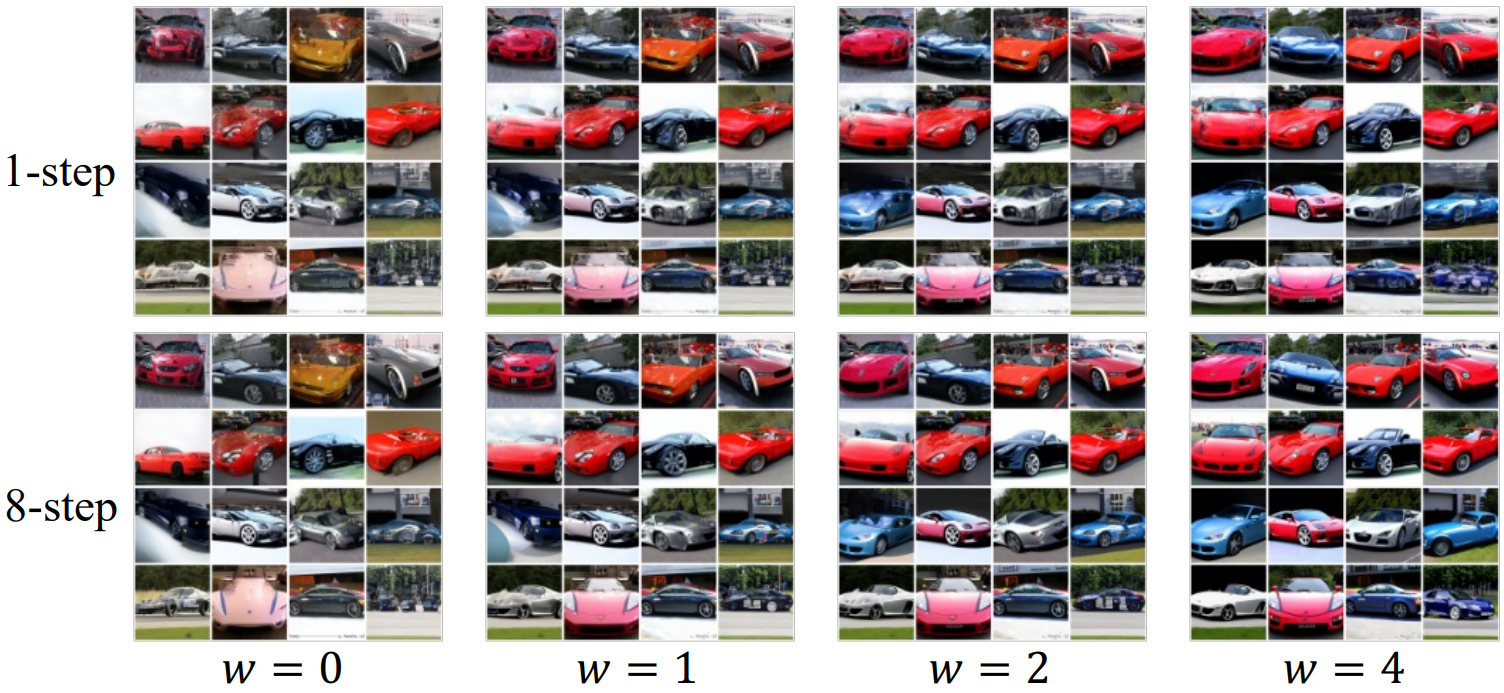
Guidance weight 파라미터 $w \in \mathbb{R}^{\ge 0}$을 사용하여 샘플 품질과 다양성 사이를 절충할 수 있다.
\[\begin{equation} \hat{x}_\theta^w = (1 + w) \hat{x}_{c, \theta} - w \hat{x}_\theta \end{equation}\]\(\hat{x}_{c, \theta}\)는 조건부 diffusion model이고 \(\hat{x}_\theta\)는 unconditional diffusion model이다. 두 모델은 공동으로 학습된다.
Distilling a guided diffusion model
Pixel-space 또는 latent-space에서 학습된 guided model(teacher)이 주어지면 본 논문의 접근 방식은 두 stage로 분해될 수 있다.
1. Stage-one distillation
첫 번째 단계에서 학습 가능한 파라미터 $\eta_1$이 있는 student model \(\hat{x}_{\eta_1} (z_t, w)\)를 도입하여 임의의 timestep $t \in [0, 1]$에서 teacher의 출력을 일치시킨다. Student model은 teacher model이 discrete인지 continuous인지에 따라 discrete-time model 또는 continuous-time model이 될 수 있다. 단순함을 위해 discrete model의 알고리즘이 continuous model의 알고리즘과 거의 동일하므로 student model과 teacher model이 모두 continuous라고 가정한다.
Classifier-free guidance의 핵심 기능은 “guidance 강도” 파라미터에 의해 제어되는 샘플 품질과 다양성 사이에서 쉽게 절충할 수 있는 능력이다. 이 속성은 최적의 “guidance 강도”가 종종 사용자 선호도인 실제 애플리케이션에서 유용성을 입증했다. 따라서 distill된 모델이 이 속성을 유지하기를 원한다. 다양한 guidance 강도 $[w_\textrm{min}, w_\textrm{max}]$를 고려하여 다음 목적 함수를 사용하여 student model을 최적화한다.
\[\begin{equation} \mathbb{E}_{w \in U[w_\textrm{min}, w_\textrm{max}], t \in U[0, 1], x \sim p_\textrm{data}(x)} [w(\lambda_t) \| \hat{x}_{\eta_1} (z_t, w) - \hat{x}_\theta^w (z_t)\|_2^2] \end{equation}\]여기에서 distill된 모델 \(\hat{x}_{\eta_1} (z_t, w)\)도 컨텍스트 $c$(ex. 텍스트 프롬프트)로 컨디셔닝되지만 단순화를 위해 $c$를 표기하지 않는다. 자세한 학습 알고리즘은 Algorithm 1과 같다.
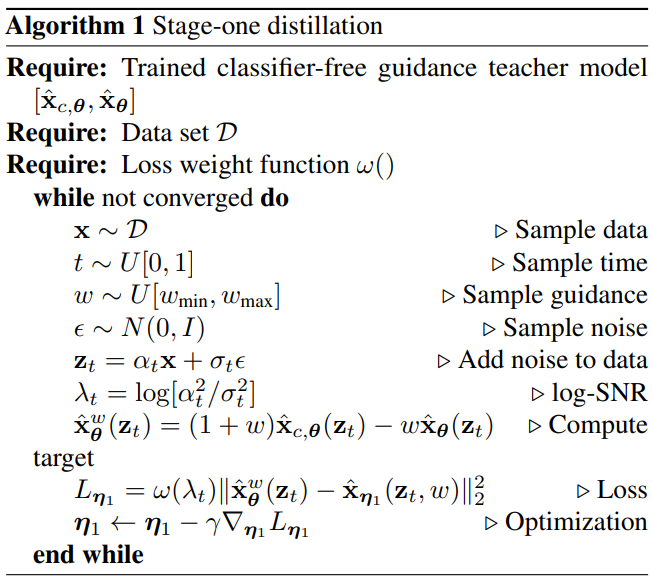
Guidance 가중치 $w$를 통합하기 위해 $w$로 컨디셔닝된 모델을 도입한다. 여기서 $w$는 student model에 대한 입력으로 공급된다. Feature를 더 잘 캡처하기 위해 푸리에 임베딩을 $w$에 적용한 다음 timestep이 통합된 방식과 유사한 방식으로 diffusion model backbone에 통합된다. 성능에서 초기화가 중요한 역할을 하기 때문에 $w$-conditioning과 관련하여 새로 도입된 파라미터를 제외하고는 teacher의 조건부 모델과 동일한 파라미터로 student model을 초기화한다. 사용하는 모델 아키텍처는 U-Net 모델이다.
2. Stage-two distillation
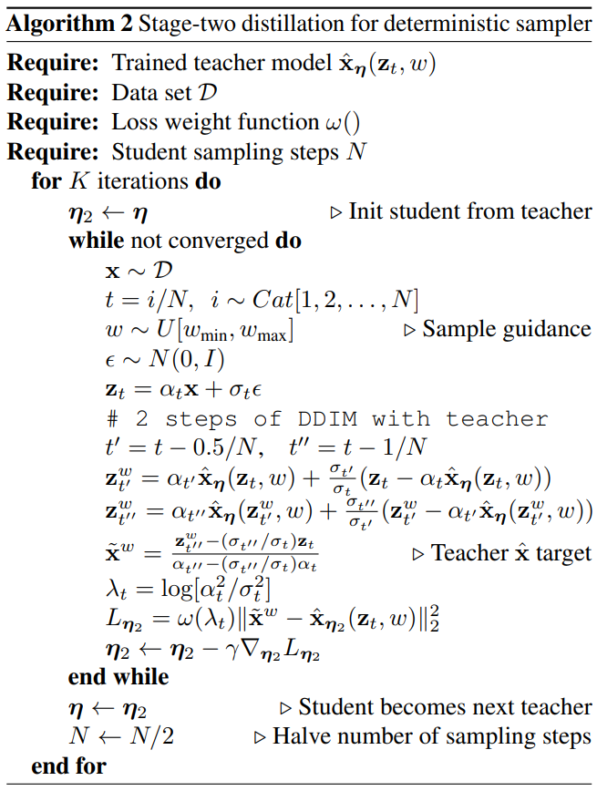
두 번째 stage에서는 discrete timestep 시나리오를 고려하고, 매번 샘플링 step 수를 반으로 줄임으로써 첫 번째 stage에서 학습된 모델 \(\hat{x}_{\eta_1} (z_t, w)\)에서 학습 가능한 파라미터 $\eta_2$를 사용하여 더 적은 step의 student model \(\hat{x}_{\eta_2} (z_t, w)\)로 점진적으로 distill한다. $N$을 샘플링 step의 수라 하고 $w \sim U[w_\textrm{min}, w_\textrm{max}]$와 \(t \in \{1, \cdots, N\}\)이 주어지면 student model을 teacher의 step 2개에 해당하는 DDIM 샘플링 출력과 일치하도록 학습시킨다. Teacher model의 $2N$ step을 student model의 $N$ step으로 distill한 후 $N$-step student model을 새로운 teacher model로 사용하고 동일한 절차를 반복하여 teacher model을 $N/2$-step student model로 distill할 수 있다. 각 step에서 teacher의 파라미터로 student model을 초기화한다.
자세한 학습 알고리즘은 Algorithm 2와 같다.
3. $N$-step deterministic and stochastic sampling
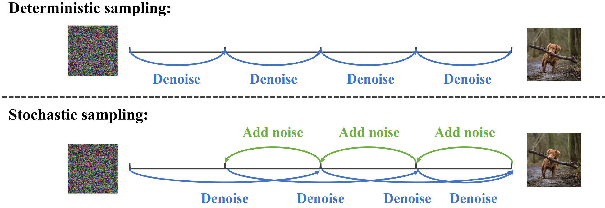
모델 \(\hat{x}_{\eta_2}\)가 학습되면 지정된 guidance 강도 $w \in [w_\textrm{min}, w_\textrm{max}]$가 주어지면 DDIM 업데이트 규칙을 통해 샘플링을 수행할 수 있다. Distiil된 모델 \(\hat{x}_{\eta_2}\)가 주어지면 이 샘플링 절차는 initialization $z_1^w$가 주어지면 deterministic하다. 실제로 $N$-step stochastic sampling도 수행할 수 있다. 원래 step 길이의 2배(즉, $N/2$-step deterministic sampler와 동일)로 하나의 deterministic sampling step을 적용한 다음 원래 step 길이를 사용하여 한 step 역방향으로 stochastic step을 수행한다. $z_1^w \sim \mathcal{N}(0,I)$에서 $t > 1/N$일 때 다음 업데이트 규칙을 사용한다.
위 식에서 $h = t - 3/N$, $k = t - 2/N$, $s = t - 1/N$이고 $\sigma_{a \vert b}^2 = (1 - e^{\lambda_a - \lambda_b}) \sigma_a^2$이다.
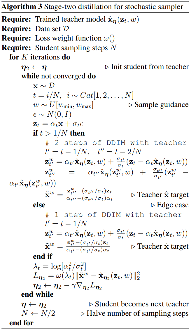
Deterministic 샘플러와 비교할 때 stochastic 샘플링을 수행하려면 약간 다른 timestep에서 모델을 평가해야 하며, edge case에 대한 학습 알고리즘을 약간 수정해야 한다. 자세한 알고리즘은 Algorithm 3과 같다.
Experiments
1. Distillation for pixel-space guided models
다음은 ImageNet 64$\times$64 샘플 품질을 나타낸 그래프이다.
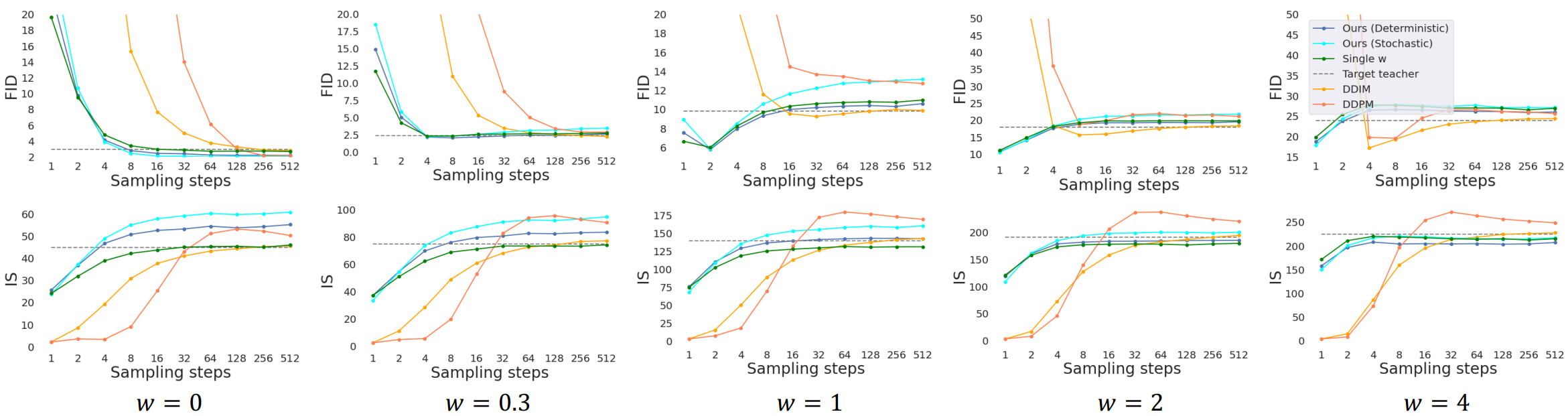
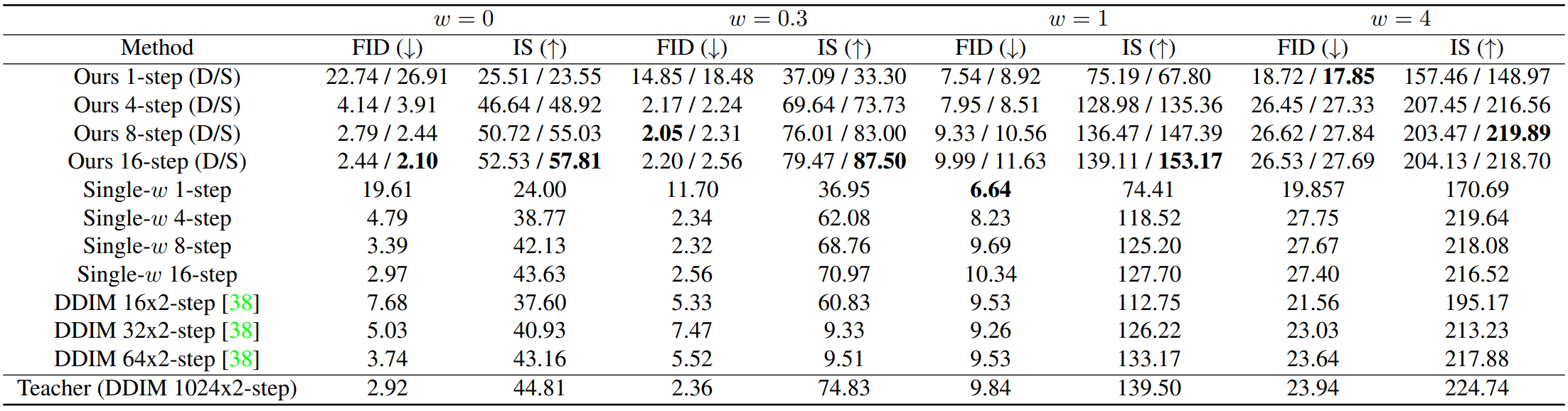
다음은 pixel-space diffusion model에 대한 ImageNet 64$\times$64 distillation 결과이다. “D”와 “S”는 각각 deterministic 샘플러와 stochastic 샘플러를 나타낸다.
2. Distillation for latent-space guided models
아래의 latent-space에 대한 실험들은 모두 distilled Stable Diffusion model을 사용하였다.
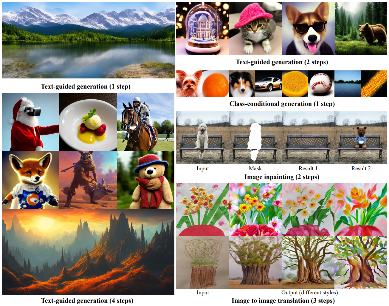
Class-conditional generation
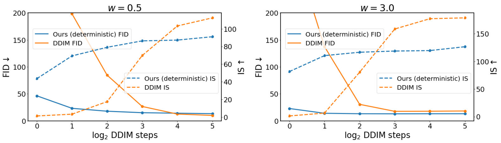
다음은 ImageNet 256$\times$256에서 클래스 조건부 이미지 생성을 평가한 그래프이다.
Text-guided image generation
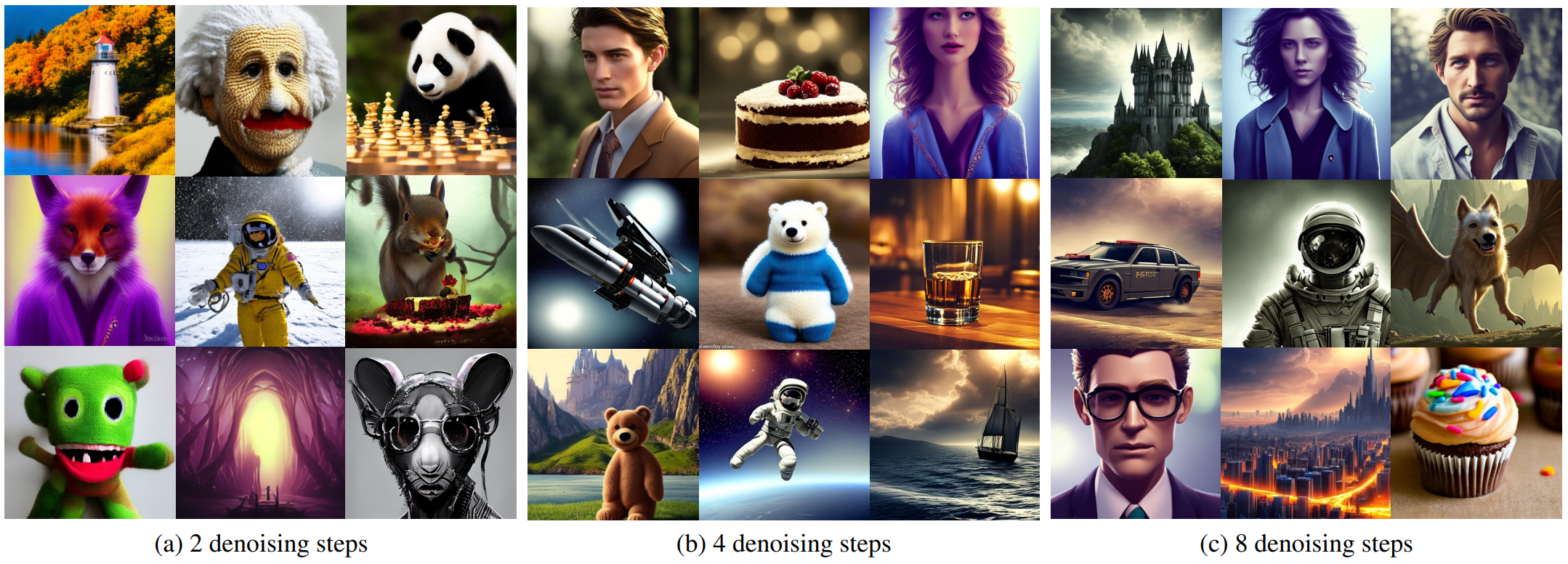
다음은 LAION (512$\times$512)에서 text-guided 생성을 한 샘플들이다.
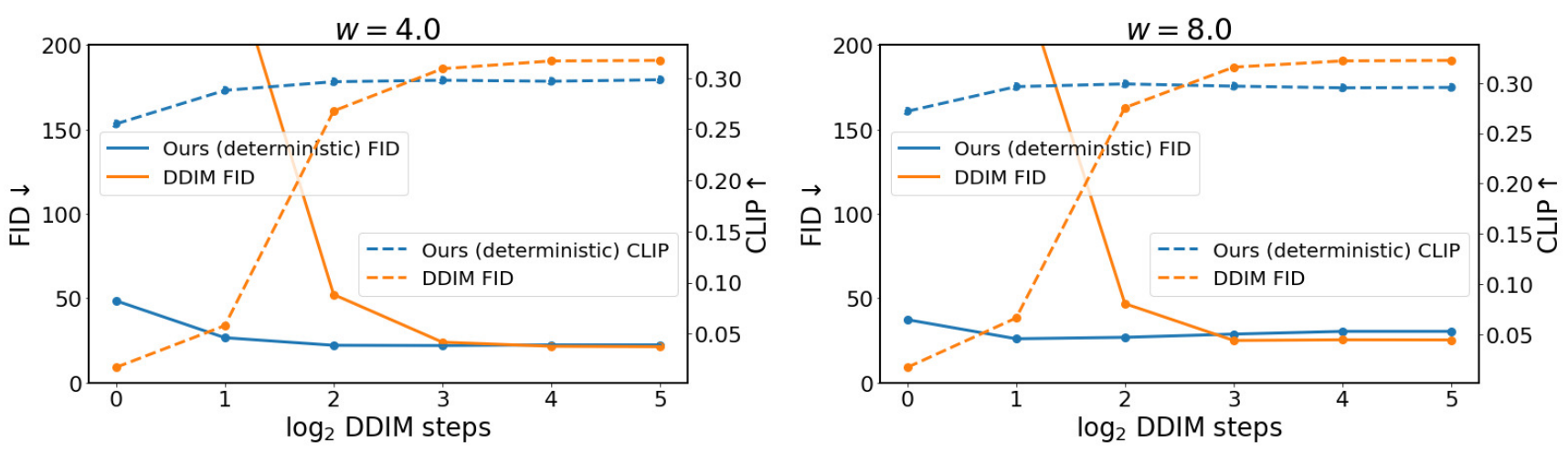
다음은 512$\times$512 text-to-image 생성을 평가한 그래프이다.
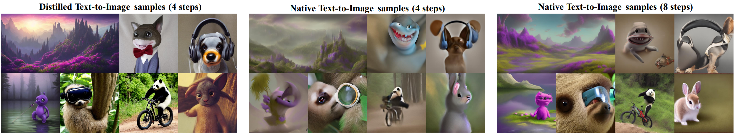
다음은 distill된 모델의 text-to-image 샘플들을 원래의 text-to-image 샘플들과 비교한 것이다.
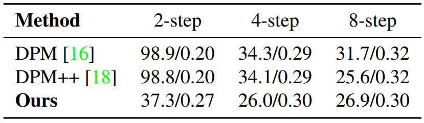
다음은 LAION 512$\times$512에서 FID와 CLIP score를 측정한 표이다.
Text-guided image-to-image translation
다음은 text-guided image-to-image translation 샘플들이다. (3 step)
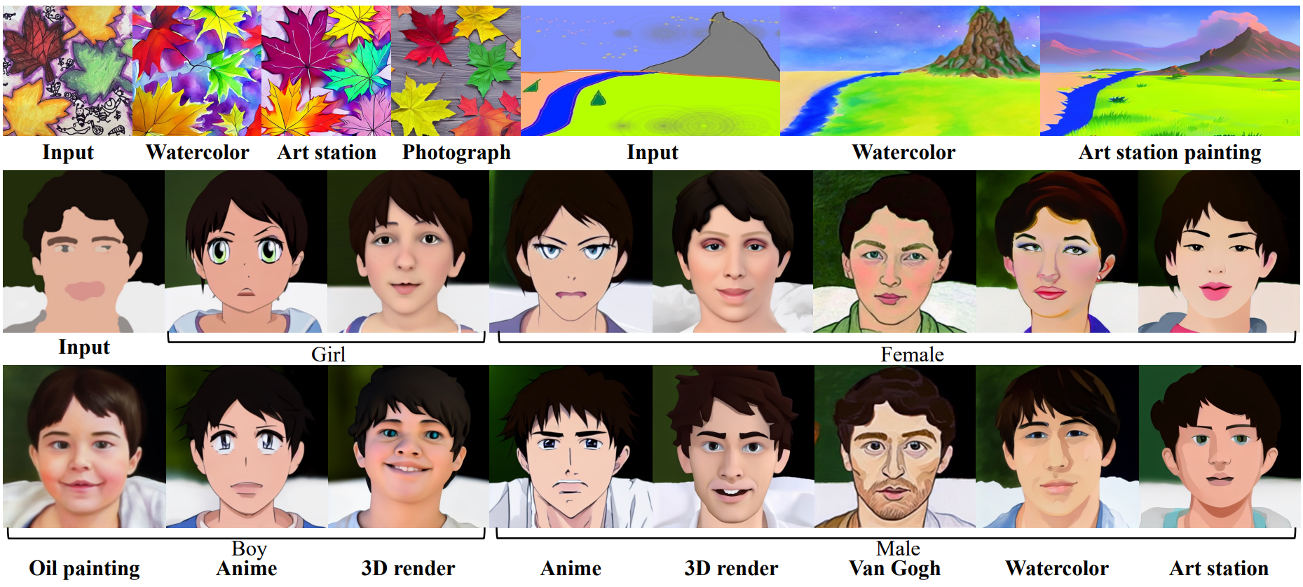
Image inpainting
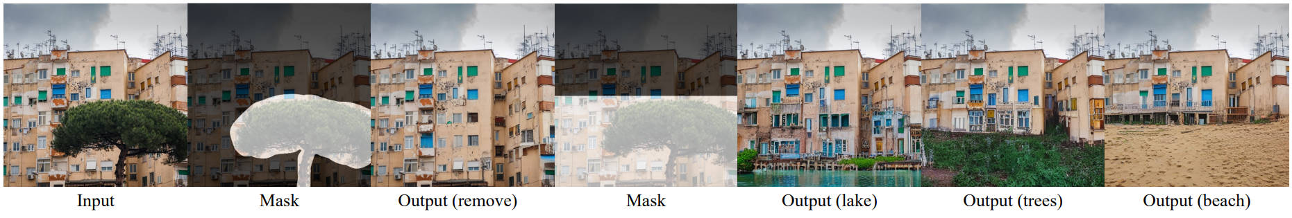
다음은 image inpainting 샘플들이다. (4 step)
3. Progressive distillation for encoding
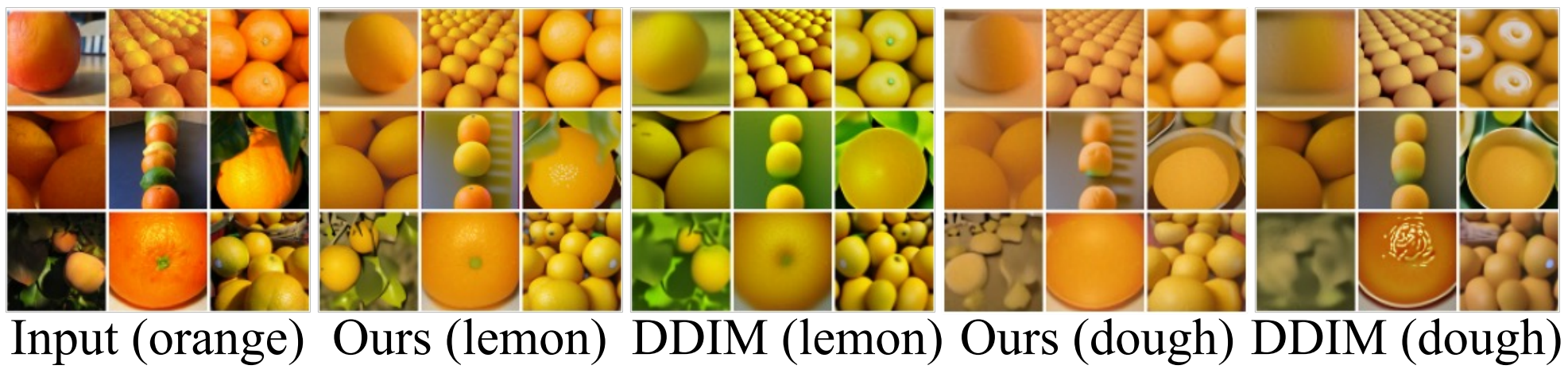
다음은 ImageNet 64$\times$64에서 pixel-space model의 style transfer를 비교한 것이다.