[논문리뷰] MapAnything: Universal Feed-Forward Metric 3D Reconstruction

arXiv 2025. [Paper] [Page] [Github]
Nikhil Keetha, Norman Müller, Johannes Schönberger, Lorenzo Porzi, Yuchen Zhang, Tobias Fischer, Arno Knapitsch, Duncan Zauss, Ethan Weber, Nelson Antunes, Jonathon Luiten, Manuel Lopez-Antequera, Samuel Rota Bulò, Christian Richardt, Deva Ramanan, Sebastian Scherer, Peter Kontschieder
Meta | Carnegie Mellon University
16 Sep 2025

Introduction

최근 연구에서는 feed-forward 아키텍처를 사용하여 이미지 기반 3D 재구성 문제를 통합된 방식으로 해결할 수 있는 엄청난 잠재력이 입증되었다. 이전 feed-forward 방법들은 서로 다른 task들을 분리하여 접근하거나 사용 가능한 모든 입력 방식을 활용하지 않은 반면, 본 논문에서는 다양한 3D 재구성 task에 대한 통합된 end-to-end 모델을 제시하였다.

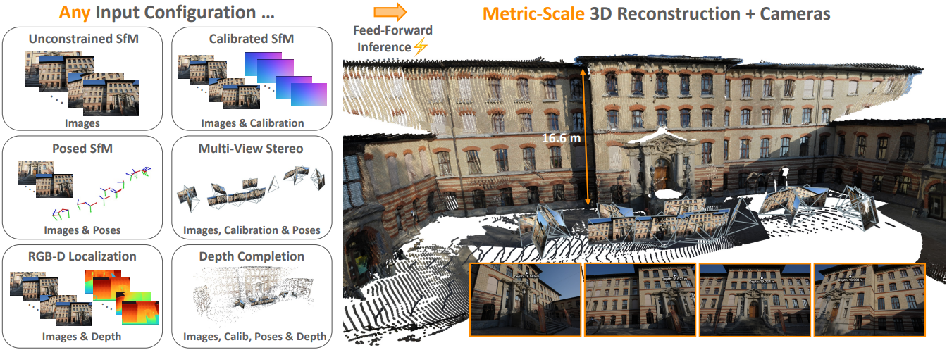
본 논문의 MapAnything은 가장 일반적인 calibration되지 않은 SfM 문제뿐만 아니라 calibration된 SfM 또는 멀티뷰 스테레오, monocular depth estimation, 카메라 위치 추정, metric depth completion 등과 같은 다양한 하위 문제 조합을 해결할 수 있다. 저자들은 이러한 통합 모델을 학습시키기 위해 다양한 geometry를 지원하는 유연한 입력 방식을 도입하고, 다양한 task를 모두 지원하는 적절한 출력 공간을 제안하였으며, 유연한 데이터셋 집계 및 표준화를 논의하였다.

MapAnything은 이러한 과제를 해결하기 위해 멀티뷰 장면 geometry를 분해하여 표현한다. 장면을 pointmap의 집합으로 직접 표현하는 대신, depth map, 로컬 ray map, 카메라 포즈, global metric scale factor의 집합으로 장면을 표현한다. 이러한 분해된 표현을 사용하여 MapAnything의 출력과 입력을 모두 표현함으로써, 사용 가능한 경우 보조 geometry 입력(ex. intrinsic, extrinsic)을 활용할 수 있도록 한다. 분해된 표현의 중요한 이점은 부분적인 주석이 있는 다양한 데이터셋, 예를 들어 metric이 아닌 “up-to-scale” geometry로만 주석이 달린 데이터셋을 통해 MapAnything을 효과적으로 학습시킬 수 있다는 것이다.

Method

MapAnything은 $N$개의 RGB 이미지 \(\hat{\mathcal{I}} = (\hat{I}_i)_{i=1}^N\)와 모든 입력 뷰 또는 일부 입력 뷰에 해당하는 선택적 geometry 입력을 입력으로 받는 end-to-end 모델이다.

1. 광선 방향 \(\hat{\mathcal{R}} = (\hat{R}_i)_{i \in S_r}\)로 나타낸 카메라 calibration
2. Quaternion \(\hat{\mathcal{Q}} = (\hat{Q}_i)_{i \in S_q}\)과 translation \(\hat{\mathcal{T}} = (\hat{T}_i)_{i \in S_t}\)로 나타낸 첫 번째 뷰 \(\hat{I}_1\)의 프레임에서의 포즈
3. 각 픽셀에 대한 광선 깊이 \(\hat{\mathcal{D}} = (\hat{D}_i)_{i \in S_d}\)

($S_r$, $S_q$, $S_t$, $S_d$는 프레임 인덱스 $[1, N]$의 부분집합)

MapAnything은 이러한 입력을 $N$-view metric 3D 출력에 매핑한다.

\[\begin{equation} f_\textrm{MapAnything} (\hat{\mathcal{I}}, [\hat{\mathcal{R}}, \hat{\mathcal{Q}}, \hat{\mathcal{T}}, \hat{\mathcal{D}}]) = \{m, (R_i, \tilde{D}_i, \tilde{P}_i)_{i=1}^N \} \text {,} (1) \end{equation}\]

($m \in \mathbb{R}$은 global metric scaling factor, $R_i \in \mathbb{R}^{3 \times H \times W}$는 예측된 로컬 광선 방향, \(\tilde{D}_i \in \mathbb{R}^{1 \times H \times W}\)는 up-to-scale space의 광선 깊이, \(\tilde{P}_i \in \mathbb{R}^{4 \times 4}\)는 \(\hat{I}_1\)의 프레임에서의 \(\hat{I}_i\)의 포즈 (quaternion $Q_i \in \textrm{SU}(2)$와 up-to-scale translation \(\tilde{T}_i \in \mathbb{R}^3\)으로 표현)

이 분해된 출력을 사용하여 up-to-scale 로컬 pointmap을 다음과 같이 얻을 수 있다.

\[\begin{equation} \tilde{L}_i = R_i \cdot \tilde{D}_i \in \mathbb{R}^{3 \times H \times W} \end{equation}\]

그런 다음, $Q_i$에서 얻은 rotation matrix $O_i \in \textrm{SO}(3)$와 up-to-scale translation \(\tilde{T}_i\)를 사용하여 world frame에서 $N$-view up-to-scale pointmap을 계산할 수 있다.

\[\begin{equation} \tilde{X}_i = O_i \cdot \tilde{L}_i + \tilde{T}_i \end{equation}\]

이미지 1의 프레임에서 $N$개의 입력 뷰에 대한 최종 metric 3D 재구성은 \(X_i^\textrm{metric} = m \cdot \tilde{X}_i\)이다.

1. Encoding Images & Geometric Inputs

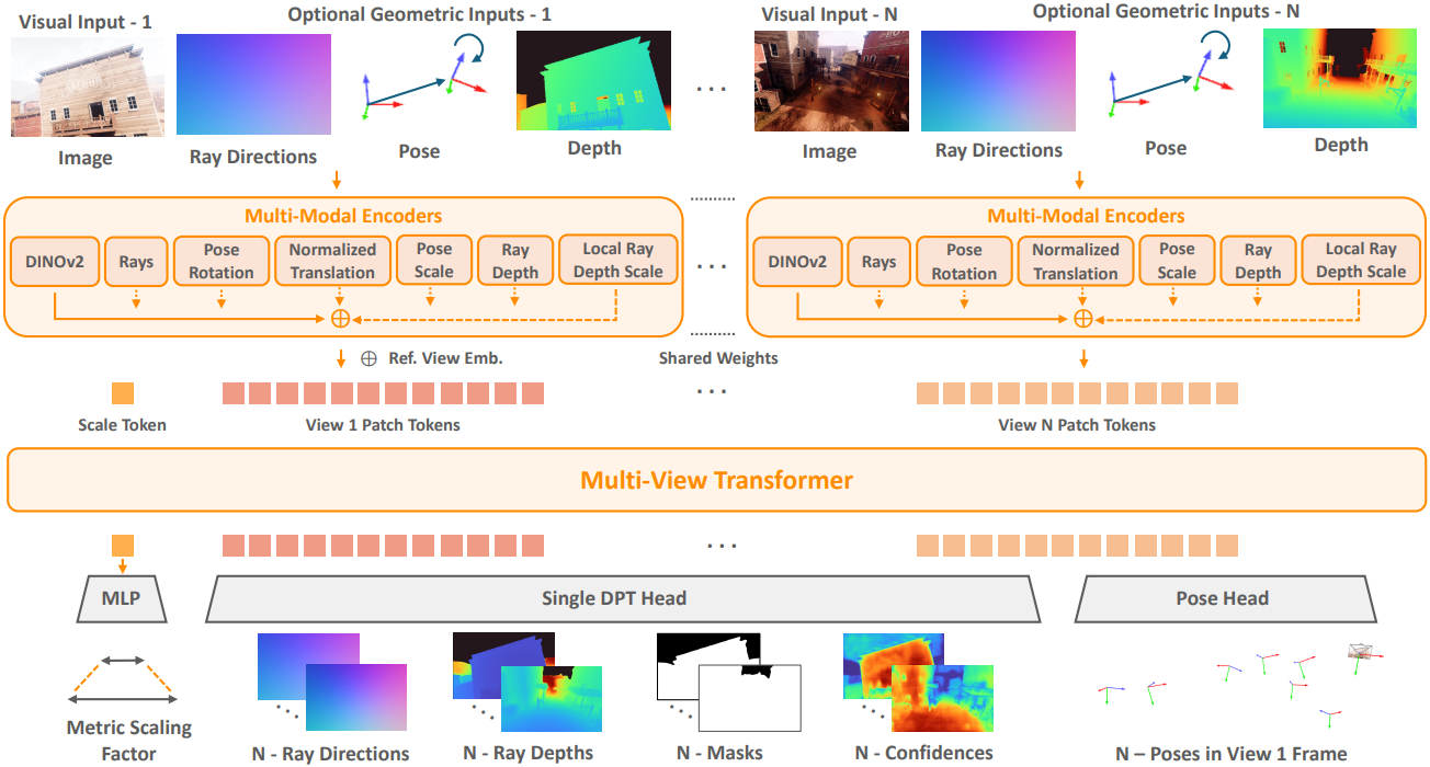
$N$개의 이미지 입력과 선택적인 dense geometry 입력을 고려하여, 먼저 이들을 공통 latent space에 인코딩한다. 이미지의 경우, 다운스트림 성능, 수렴 속도, 일반화 측면에서 뛰어난 DINOv2를 사용한다. DINOv2 ViT-L 마지막 레이어의 정규화된 패치 feature $F_I$를 사용한다.

\[\begin{equation} F_I \in \mathbb{R}^{1024 \times H/14 \times W/14} \end{equation}\]

MapAnything은 다른 geometry 값들도 인코딩할 수 있다. 이러한 geometry 값들을 네트워크에 공급하기 전에, metric 값과 up-to-scale 값 모두에 대한 학습 및 inference를 가능하게 하기 위해 이를 분해한다. 특히, 광선 깊이가 제공되면, 광선 깊이는 먼저 평균 깊이 \(\hat{z}_{di} \in \mathbb{R}^{+}\)와 정규화된 광선 깊이 \(\hat{D}_i / \hat{z}_{di}\)로 분리된다. 또한, translation $\hat{\mathcal{T}}$가 제공되면 MapAnything은 world frame까지의 평균 거리 \(\hat{z}_p\)로 포즈 scale을 계산한다.

\[\begin{equation} \hat{z}_p = \frac{1}{\vert S_t \vert} \sum_{i \in S_t} \| \hat{T}_i \| \end{equation}\]

이 포즈 scale은 입력 translation이 있는 모든 프레임에 대해 동일한 입력으로 사용되며, 정규화된 translation \(\hat{T}_i / \hat{z}_p\)를 얻는 데에도 사용된다. Geometry 입력에서 metric scale 정보를 효과적으로 활용하는 데 관심이 있으므로, MapAnything은 특정 프레임에 제공된 포즈와 깊이가 metric일 때만 포즈 scale과 깊이 scale을 사용한다. Metric scale 값은 크거나 장면 크기에 따라 크게 달라질 수 있으므로 인코딩하기 전에 scale에 로그 변환을 수행한다.

공간적 resizing이 크기 14의 pixel unshuffle에서 한 번만 발생하는 얕은 convolution 인코더를 사용하여 광선 방향과 정규화된 광선 깊이를 인코딩한다. 이를 통해 dense한 geometry 입력을 DINOv2 feature와 동일한 공간 및 latent 차원으로 projection한다.

\[\begin{equation} F_R, F_D \in \mathbb{R}^{1024 \times H/14 \times W/14} \end{equation}\]

글로벌한 non-pixel 값들, 즉 quaternion으로 표현되는 rotation, translation 방향, 깊이 scale, 포즈 scale의 경우 GeLU activation을 사용하는 4-layer MLP를 사용하여 값들을 feature로 projection한다.

\[\begin{equation} F_Q, F_T, F_{\hat{z}_d}, F_{\hat{z}_p} \in \mathbb{R}^{1024} \end{equation}\]

모든 입력 값들이 인코딩되면 layer normalization을 거친 후 더해지고, 이어서 또 다른 layer normalization을 거쳐 각 입력 뷰에 대한 최종 뷰별 인코딩을 얻는다. 그런 다음, 이것들은 토큰 $F_E$로 flatten된다.

\[\begin{equation} F_E \in \mathbb{R}^{1024 \times (HW / 256)} \end{equation}\]

저자들은 $N$개의 뷰 패치 토큰들에 하나의 학습 가능한 scale 토큰을 추가하고 토큰을 multi-view transformer에 입력하여 여러 뷰에 걸친 정보가 서로 attention하고 정보를 전파할 수 있도록 하였다. Multi-view transformer는 레이어가 24개인 alternating-attention transformer이며, multi-head attention의 head는 12개, latent 차원은 768, MLP ratio는 4이다. 레퍼런스 뷰, 즉 첫 번째 뷰를 구별하기 위해 첫 번째 뷰에 해당하는 패치 토큰 세트에 상수 레퍼런스 뷰 임베딩을 추가한다. 또한, 더 간단하게 하기 위해 Rotary Positional Embedding (RoPE)을 사용하지 않으며, 이는 DINOv2의 패치 수준의 위치 인코딩이 충분하고 RoPE를 사용하였을 때 불필요한 편향으로 이어지는 경향이 있기 때문이다.

2. Factored Scene Representation Prediction

Multi-view transformer가 여러 뷰에 걸쳐 정보를 융합하고 $N$-view 패치 토큰과 scale 토큰을 출력하면 MapAnything은 이러한 토큰을 추가로 디코딩하여 metric 3D geometry를 나타내는 값들로 변환한다. 특히, DPT head를 사용하여 $N$-view 패치 토큰을 $N$개의 dense한 뷰별 출력, 즉 광선 방향 $R_i$ (단위 길이로 정규화), up-to-scale 광선 깊이 \(\tilde{D}_i\), 모호하지 않은 깊이를 나타내는 마스크 $M_i$, 신뢰도 맵 $C_i$로 디코딩한다.

또한, $N$-view 패치 토큰을 average pooling 기반 convolutional head에 입력하여 unit quaternion $Q_i$와 up-to-scale translation \(\tilde{T}_i\)를 예측한다. Scale 토큰은 ReLU를 사용한 2-layer MLP를 통과하여 metric scaling factor $m$이 예측된다. 장면의 metric scale은 매우 다양할 수 있으므로 예측을 지수적으로 scaling하여 $m$을 얻는다. 이러한 분리된 예측들을 함께 사용하여 metric 3차원 재구성을 얻을 수 있다.

3. Training Universal Metric 3D Reconstruction

사용 가능한 supervision에 따라 여러 loss를 사용하여 MapAnything을 end-to-end로 학습시킨다. 광선 방향 $R_i$와 포즈 quaternion $Q_i$는 장면 scale에 의존하지 않으므로 loss는 다음과 같다.

\[\begin{aligned} \mathcal{L}_\textrm{rays} &= \sum_{i=1}^N \| \hat{R}_i - R_i \| \\ \mathcal{L}_\textrm{rot} &= \sum_{i=1}^N \min (\| \hat{Q}_i - Q_i \|, \| -\hat{Q}_i - Q_i \|) \end{aligned}\]

이는 unit quaternion의 2:1 매핑을 설명하며, regression loss는 geodesic angular distance와 유사하다.

예측된 up-to-scale 값들을 위해, DUSt3R를 따라 GT와 up-to-scale 예측에 대한 scaling factor를 각각 계산한다.

\[\begin{equation} \hat{z} = \frac{\| (\hat{X}_i [V_i])_{i=1}^N \|}{\sum_{i=1}^N V_i}, \quad \tilde{z} = \frac{\| (\tilde{X}_i [V_i])_{i=1}^N \|}{\sum_{i=1}^N V_i} \end{equation}\]

($V_i$는 GT validity mask)

마찬가지로 scale loss로 인한 gradient가 geometry에 영향을 미치지 않도록, 예측된 $m$과 계산된 $\tilde{z}$를 사용하여 다음과 같이 metric norm scaling factor를 계산한다.

\[\begin{equation} z^\textrm{metric} = m \cdot \textrm{stop-grad} (\tilde{z}) \end{equation}\]

Scaling factor를 사용하여 scale-invariant translation loss를 계산할 수 있다.

\[\begin{equation} \mathcal{L}_\textrm{translation} = \sum_{i=1} \| \frac{\hat{T}_i}{\hat{z}} - \frac{\tilde{T}_i}{\tilde{z}} \| \end{equation}\]

광선 깊이, pointmap, metric scaling factor에 대해 log-space에서 loss를 적용하는 것이 중요하기 때문에, \(f_\textrm{log}\)를 사용하여 log-space로 변환 후에 loss를 적용한다.

\[\begin{equation} f_\textrm{log} (\textbf{x}) = \frac{\textbf{x}}{\| \textbf{x} \|} \cdot \log (1 + \| \textbf{x} \|) \end{equation}\]

따라서, 광선 깊이 \(\tilde{D}_i\)에 대한 loss \(\mathcal{L}_\textrm{depth}\)와 로컬 pointmap \(\tilde{L}_i\)에 대한 loss \(\mathcal{L}_\textrm{lpm}\)은 다음과 같이 계산된다.

\[\begin{aligned} \mathcal{L}_\textrm{depth} &= \sum_{i=1}^N \| f_\textrm{log} (\frac{\hat{D}_i}{\hat{z}}) - f_\textrm{log} (\frac{\tilde{D}_i}{\tilde{z}}) \| \\ \mathcal{L}_\textrm{lpm} &= \sum_{i=1}^N \| f_\textrm{log} (\frac{\hat{L}_i}{\hat{z}}) - f_\textrm{log} (\frac{\tilde{L}_i}{\tilde{z}}) \| \end{aligned}\]

학습 데이터의 불완전성과 잠재적 outlier를 무시하기 위해 픽셀별 loss 값의 상위 5%를 제외한다. World frame pointmap \(\tilde{X}_i\)의 경우, DUSt3R의 신뢰도 기반 pointmap loss를 추가한다.

\[\begin{equation} \mathcal{L}_\textrm{pointmap} = \sum_{i=1}^N C_i \| f_\textrm{log} (\frac{\hat{X}_i}{\hat{z}}) - f_\textrm{log} (\frac{\tilde{X}_i}{\tilde{z}}) \| - \alpha \log C_i \end{equation}\]

Metric scale loss는 다음과 같다.

\[\begin{equation} \mathcal{L}_\textrm{scale} = \| f_\textrm{log} (\hat{z}) - f_\textrm{log} (z^\textrm{metric}) \| \end{equation}\]

미세한 디테일을 포착하기 위해, 로컬 pointmap에 normal loss \(\mathcal{L}_\textrm{normal}\)을 적용하고, 로컬 pointmap의 z-depth의 로그 값에 multi-scale gradient matching loss \(\mathcal{L}_\textrm{GM}\)을 적용한다. 실제 데이터셋의 geometry는 coarse하고 노이즈가 많을 수 있으므로, 합성 데이터셋에만 \(\mathcal{L}_\textrm{normal}\)과 \(\mathcal{L}_\textrm{GM}\)을 적용한다. 예측된 $M$에는 binary cross entropy loss \(\mathcal{L}_\textrm{mask}\)를 사용한다.

전체적으로 다음과 같은 loss를 사용한다.

\[\begin{aligned} \mathcal{L} &= 10 \cdot \mathcal{L}_\textrm{pointmap} + \mathcal{L}_\textrm{rays} + \mathcal{L}_\textrm{rot} + \mathcal{L}_\textrm{translation} + \mathcal{L}_\textrm{depth} \\ & \quad + \mathcal{L}_\textrm{lpm} + \mathcal{L}_\textrm{scale} + \mathcal{L}_\textrm{normal} + \mathcal{L}_\textrm{GM} + 0.1 \cdot \mathcal{L}_\textrm{mask} \end{aligned}\]

모든 regression loss의 경우, inlier를 개선하기 위해 adaptive robust loss ($c = 0.05$, $\alpha = 0.5$)를 사용한다.

Experiments

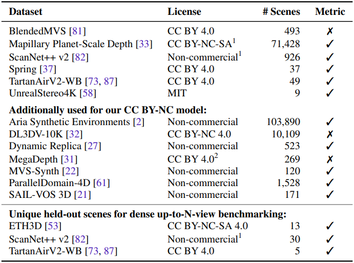
학습에 사용된 데이터셋들은 아래 표와 같다.

1. Multi-View Dense Reconstruction

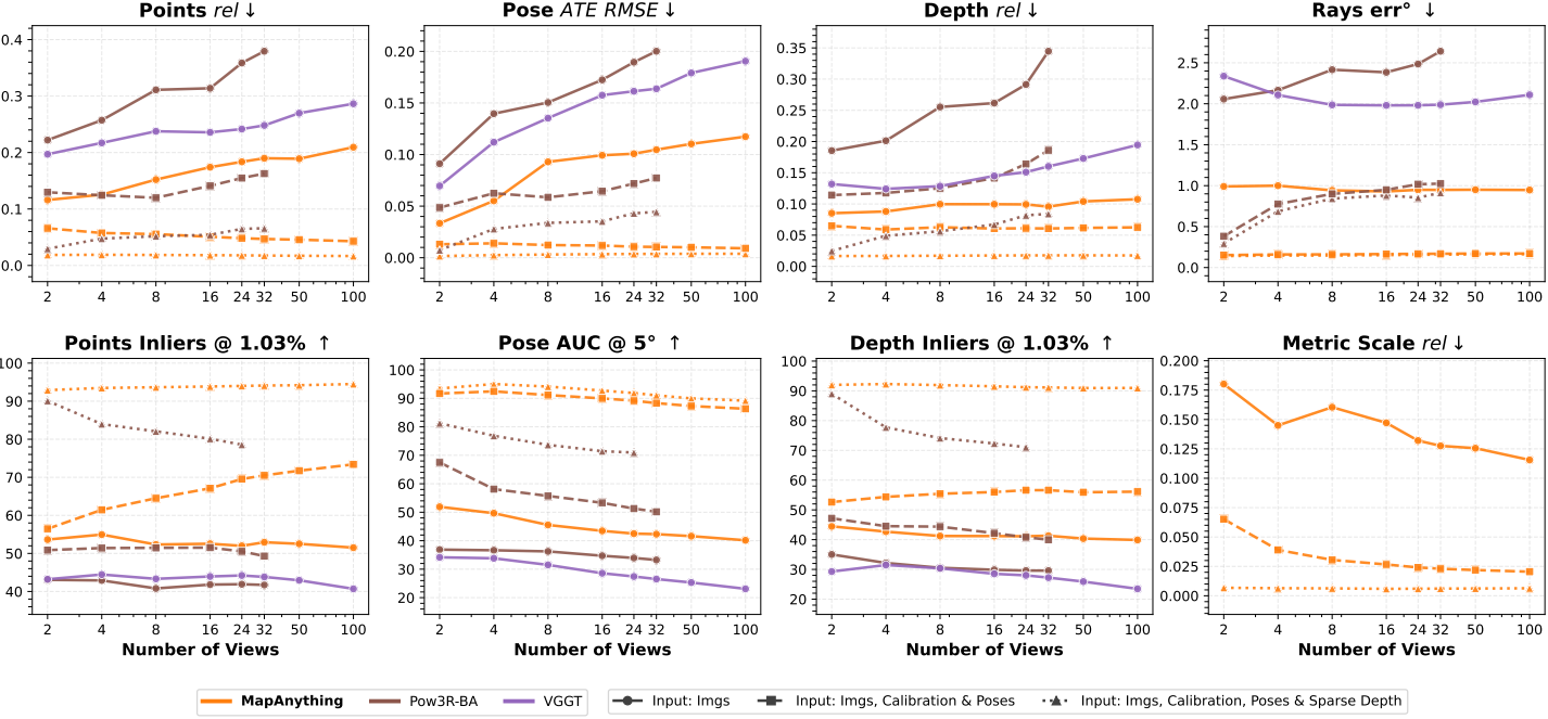
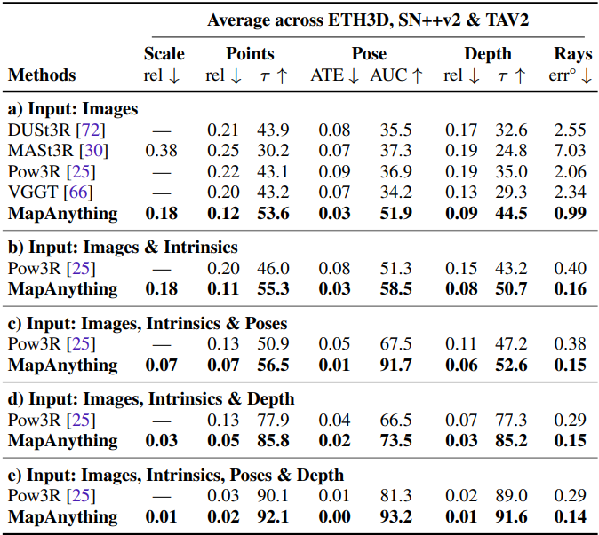
다음은 입력 뷰 수에 따른 멀티뷰 재구성 성능을 비교한 결과이다.

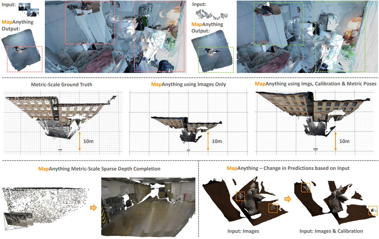
다음은 보조 geometry 입력 유무에 따른 MapAnything 성능 차이를 비교한 예시들이다.

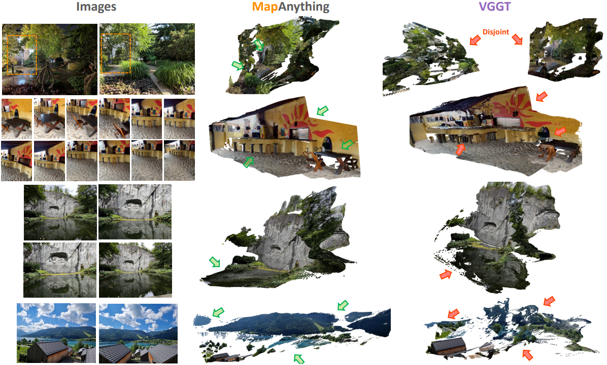
다음은 VGGT와 in-the-wild 이미지들에 대하여 비교한 결과이다.

2. Two-View Dense Reconstruction

다음은 2-view 재구성 성능을 비교한 결과이다.

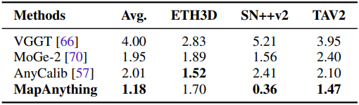
3. Single-View Calibration

다음은 단일 이미지 기반 calibration 성능을 비교한 결과이다.

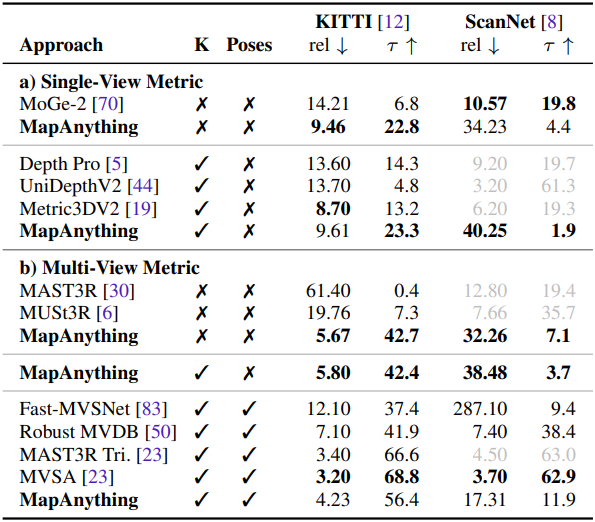
4. Monocular & Multi-View Depth Estimation

다음은 metric depth estimation 성능을 비교한 결과이다.

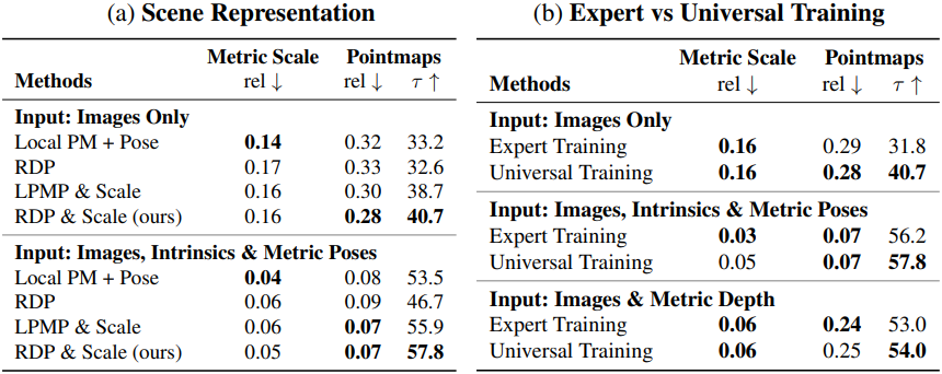
5. Insights into enabling MapAnything

다음은 ablation study 결과이다.

6. Qualitative Examples

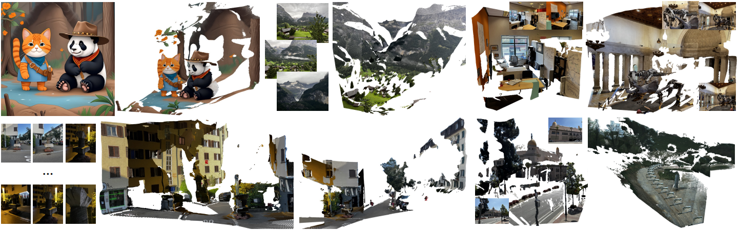
다음은 3D 재구성 예시들이다.