[논문리뷰] Lavender: Diffusion Instruction Tuning
ICML 2025. [Paper] [Page] [Github]
Chen Jin, Ryutaro Tanno, Amrutha Saseendran, Tom Diethe, Philip Teare
AstraZeneca | Google DeepMind
4 Feb 2025
Introduction
정밀한 비전-텍스트 정렬은 고급 멀티모달 추론에 필수적이다. Vision-language model(VLM)과 diffusion model(DM)은 모두 텍스트와 이미지를 처리하지만, 서로 다른 loss를 사용한다. 픽셀 레벨에서 이미지를 재구성하는 DM은 텍스트 토큰 생성에만 최적화된 VLM보다 더 정밀한 텍스트-비전 attention map을 학습한다.
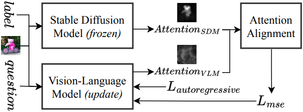
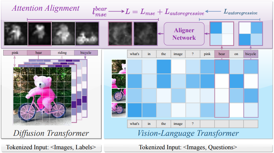
본 논문에서는 VLM transformer attention layer를 Stable Diffusion attention layer와 직접 정렬하는 최초의 프레임워크인 Lavender를 소개한다. DM에서 추출한 고품질 cross-attention map은 supervised fine-tuning (SFT) 동안 VLM의 텍스트-비전 attention 유도에 유용한 타겟을 제공하여 word-to-region 정렬 및 전반적인 성능을 향상시킨다. 또한, catastrophic forgetting을 완화하기 위해 기존 VLM 역량을 보존하는 여러 attention 집계 방법과 학습 전략을 제안하였다.
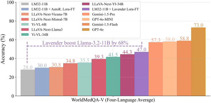
작은 OpenFlamingo 모델에서 Lavender를 검증한 결과, Lavender가 VLM attention을 DM attention과 일치시키는 것으로 나타났다. Lavender는 20가지 다양한 벤치마크에서 autoregressive fine-tuning보다 눈에 띄는 성과를 보였으며, 그중 7가지 벤치마크에서 OpenFlamingo 대비 최대 70%의 성능 향상을 보였다. Fine-tuning된 Llama 3.2-11B의 경우, 19가지 벤치마크에서 성능이 최대 30% 향상되어 유사한 소규모 오픈소스 모델보다 50% 더 뛰어나다. 이러한 장점은 매우 극심한 out-of-distribution (OOD) 도메인으로도 확장되어, WorldMedQA 벤치마크에서의 성능을 68% 향상시켰다.
Diffusion Instruction Tuning
사전 학습된 diffusion model(DM)의 attention 분포를 활용하여 사전 학습된 VLM을 향상시키고자 한다. VLM 성능을 극대화하는 이상적인 attention 분포가 존재하며, DM의 attention이 이 이상적인 분포에 더 가깝다고 가정한다.
Notation
- 이미지: $x$, 질문: $y_q$, 정답 레이블: $y_l$
- 파라미터가 $\theta$인 VLM은 $p(y_l \vert x, y_q; \theta)$를 모델링
- 파라미터가 \(\theta_D\)인 DM은 \(p(x \vert y; \theta_D)\)를 모델링
- Attention 분포는 각각 \(p_\textrm{VLM} (a \vert x, y; \theta)\), \(p_\textrm{DM} (a \vert x, y; \theta_D)\)
DM 파라미터 \(\theta_D\)를 고정해두고, 사전 학습된 VLM 파라미터 $\theta$만 fine-tuning한다.
1. Bayesian Derivation
Posterior Distribution
데이터 $D$와 DM의 attention 분포를 고려하여 VLM 파라미터의 posterior 분포를 찾는 것을 목표로 한다.
\[\begin{equation} p (\theta \vert D, A_\textrm{DM}) \propto p (D \vert \theta) p (A_\textrm{DM} \vert \theta) p(\theta) \end{equation}\](\(A_\textrm{DM} = \{p_\textrm{DM} (a \vert x^{(i)}, y^{(i)}; \theta_D)\}\)는 DM의 조건부 분포에서 파생된 attention 출력의 컬렉션, $p(\theta)$는 VLM 파라미터에 대한 prior)
Likelihood of the Data
주어진 $\theta$에 대한 데이터의 likelihood는 다음과 같다.
\[\begin{equation} p (D \vert \theta) = \prod_i p (y_l^{(i)} \vert x^{(i)}, y_q^{(i)}; \theta) \end{equation}\]VLM을 fine-tuning하는 데 negative log-likelihood (NLL)에 해당하는 loss function \(L_\textrm{VLM} (\theta)\)가 사용된다.
\[\begin{equation} L_\textrm{VLM} (\theta) = - \sum_i \log p (y_l^{(i)} \vert x^{(i)}, y_q^{(i)}; \theta) \end{equation}\]Likelihood of the DM’s Attention
주어진 VLM 파라미터에 대하여 DM의 attention을 관찰할 likelihood \(p(A_\textrm{DM} \vert \theta)\)를 모델링한다. 표기법을 단순화하고 방정식을 더 간결하게 만들기 위해 $\delta^{(i)} (\theta)$를 도입한다.
\[\begin{equation} \delta^{(i)} (\theta) = p_\textrm{VLM} (a \vert x^{(i)}, y^{(i)}; \theta) - p_\textrm{DM} (a \vert x^{(i)}, y^{(i)}; \theta_D) \end{equation}\]이는 $i$번째 데이터 포인트에 대한 VLM과 DM의 attention 분포 간의 데이터 포인트별 차이를 나타내며, 각 attention 위치 $a$에서의 발산에 대한 측정치 역할을 한다. 이 차이가 동일한 분산을 가지는 Gaussian 분포를 따른다고 가정하면, likelihood는 다음과 같이 표현될 수 있다.
\[\begin{equation} p(A_\textrm{DM} \vert \theta) \propto \exp \left( - \frac{\lambda}{2} \sum_i \| \delta^{(i)} (\theta) \|^2 \right) \end{equation}\]이는 attention 정렬 loss \(L_\textrm{att}(\theta)\)에 해당한다.
\[\begin{equation} L_\textrm{att} (\theta) = \sum_i \| \delta^(i) (\theta) \|^2 \end{equation}\]이 MSE loss를 최소화함으로써 VLM의 attention이 DM의 attention과 일치하도록 하여 최적의 posterior attention 분포 \(p^\ast (a \vert x, y)\)를 향하도록 유도한다.
단순화를 위해, non-informative prior $p(\theta)$를 가정한다. 결과적으로, posterior 분포 \(p(\theta \vert D, A_\textrm{DM})\)는 주로 \(p(D \vert \theta)\)와 \(p (A_\textrm{DM} \vert \theta)\)에 의해 결정된다. 이 두 항을 결합하면, negative log-posterior는 다음과 같다.
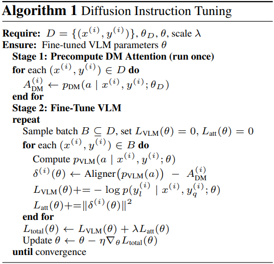
\[\begin{equation} L_\textrm{total} (\theta) = L_\textrm{VLM} (\theta) + \lambda L_\textrm{att} (\theta) \end{equation}\]2. Interpretation and Practical Implementation
\(L_\textrm{total} (\theta)\)을 최소화함으로써 \(p(\theta \vert D, A_\textrm{DM})\)을 최대화하여 VLM의 attention을 이상적인 posterior \(p^\ast (a \vert x, y)\)에 더 가깝게 정렬한다. 이를 통해 VLM이 텍스트 토큰을 관련 시각적 영역과 연관시키는 능력이 향상되어 비전-텍스트 이해도가 향상된다.
이를 구현하기 위해 사전 학습된 DM과 VLM에서 단어별 attention 분포를 추출한다.
\[\begin{equation} p_\textrm{DM} (a \vert x^{(i)}, y^{(i)}; \theta_D), \quad p_\textrm{VLM} (a \vert x^{(i)}, y^{(i)}; \theta) \end{equation}\]Fine-tuning은 다음을 최소화한다.
\[\begin{equation} L_\textrm{total} (\theta) = - \sum_i \log p (y_l^{(i)} \vert x^{(i)}, y_q^{(i)}; \theta) + \lambda \sum_i \| \delta^{(i)} (\theta) \|^2 \end{equation}\]이 모델 독립적인 프로세스는 추가 데이터가 필요하지 않으며 다양한 VLM 아키텍처에서 작동한다.
Attention Alignment
1. Attention Aggregation in Diffusion Models
텍스트 기반 diffusion model은 랜덤 noise 이미지를 반복적으로 denoising하여 텍스트 입력으로부터 이미지를 생성한다. 각 denoising step에서 cross-attention layer는 모델이 관련 텍스트 토큰에 집중할 수 있도록 한다. 구체적으로, query $Q$는 noise가 더해진 이미지 $x_t$에서 도출되고, key $K$와 value $V$는 텍스트 임베딩 $v$에서 도출된다.
\[\begin{equation} Q = f_Q (x_t), \quad K = f_K (v), \quad V = f_V (v) \end{equation}\]($f_Q$, $f_K$, $f_V$는 DM의 사전 학습된 projection 행렬)
Attention map $M$은 다음과 같이 계산된다.
\[\begin{equation} M = \textrm{Softmax} ( \frac{QK^\top}{\sqrt{d}} ) \end{equation}\]2. Attention Aggregation in Vision-Language Models
VLM은 transformer attention을 사용하여 여러 head와 layer에 걸쳐 텍스트 토큰 $T_t$와 이미지 패치 토큰 $T_p$를 연결하여 attention 가중치 \(w_{t,p}^{hl}\)를 형성한다. 여기서 $h$, $l$, $t$, $p$는 각각 head, layer, 토큰, 패치를 나타낸다. 이러한 가중치는 토큰과 패치 간의 semantic 관계와 공간적 관계를 포착한다.
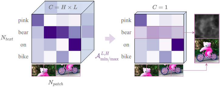
단어별 saliency map을 생성하기 위해, 먼저 모든 head와 layer에 걸쳐 attention을 집계하여 \((N_\textrm{text} \times N_\textrm{patch} \times H \times L)\) 텐서를 \((N_\textrm{text} \times N_\textrm{patch})\) 행렬로 축소시킨다. 그런 다음, 이 행렬을 \(\sqrt{N_\textrm{patch}} \times \sqrt{N_\textrm{patch}}\) 그리드로 재구성하여 원본 이미지의 공간적 레이아웃을 대략적으로 재구성한다.
이 과정을 통해 해석 가능한 saliency map이 생성되며, 각 행은 텍스트 토큰이 이미지 패치에 어떻게 초점을 맞추는지 강조한다. 이러한 saliency map을 통해 VLM attention을 DM attention과 일치시킬 수 있다. 저자들은 VLM에 가장 적합한 attention 집계 메커니즘을 탐색하기 위해 다양한 접근 방식을 사용하였다.
Simple aggregation functions
간단한 접근 방식은 평균 또는 최대값을 통해 head $H$와 layer $L$에 걸쳐 attention 가중치 $\textbf{A}$, 즉 \(w_{t,p}^{hl}\)를 pooling하는 것이다. 저자들은 4가지 전략을 고려하였다.
\[\begin{equation} \mathcal{A}_\textrm{mean/max}^{(L, H)} (\textbf{A}) \in \{ \textrm{max-mean}, \textrm{max-mean}, \textrm{mean-max}, \textrm{mean-mean} \} \end{equation}\]각각은 $H$와 $L$에 대한 \(\{\textrm{Max}, \textrm{Mean}\}\)의 조합을 나타낸다. 이를 통해 단어별 attention map이 생성되어 단어와 패치의 정렬을 대략적으로 측정할 수 있다.
Attention flow
Attention flow는 여러 layer에 걸쳐 attention을 축적하여 정보가 네트워크를 통해 어떻게 전파되는지 추적한다. 단순 pooling과 달리, 이 방법은 모든 layer를 함께 고려하여 더 깊은 의존성을 포착한다.
여러 layer 간의 상호작용을 포착하기 위해 attention map을 재귀적으로 업데이트한다. 첫 번째 layer의 attention $A^{(1)}$부터 시작하여, 이후 각 layer의 attention $A^{(l)}$을 element-wise multiplication 또는 element-wise addition을 사용하여 병합한다.
\[\begin{equation} \bar{A} \leftarrow \bar{A} \circ A^{(l)} \quad \textrm{or} \quad \bar{A} \leftarrow \bar{A} + A^{(l)} \end{equation}\]이 방법은 여러 layer에 걸쳐 attention을 통합함으로써, 기존 방법들이 간과하는 semantic 관계를 강조할 수 있다.
Learning the attention aggregations
표준 접근법은 미리 정의된 pooling 방법을 사용하여 attention을 집계하는데, 이는 세밀한 관계를 잃을 수 있다. 대신, 사전 학습된 projection $(W_Q, W_K)$와 함께 병렬 cross-attention 파라미터 $(W_{Q_d}, W_{K_d})$를 도입한다. 이를 통해 기존 가중치를 덮어쓰지 않고도 더욱 풍부한 semantic 상관관계를 포착할 수 있다.
사전 학습된 attention의 이점을 유지하면서도 새롭게 학습된 패턴을 통합하기 위해, 각 forward pass 동안 원래 attention $A$와 병렬 attention $A_d$를 모두 계산한다. 그런 다음 병렬 attention $A_d$를 사용하여 DM과 정렬한다.
\[\begin{equation} A = \textrm{Softmax} (\frac{QK^\top}{\sqrt{d_k}}), \quad A_d = \textrm{Softmax} (\frac{Q_d K_d^\top}{\sqrt{d_k}}) \end{equation}\]경험적으로, layer의 1/5만 병렬 cross-attention을 학습하는 것만으로도 효과적인 정렬에 충분하다. 이 접근법은 효율성과 정확성의 균형을 이루며, VLM의 핵심 지식을 보존하는 동시에 DM의 attention 분포를 활용한다.
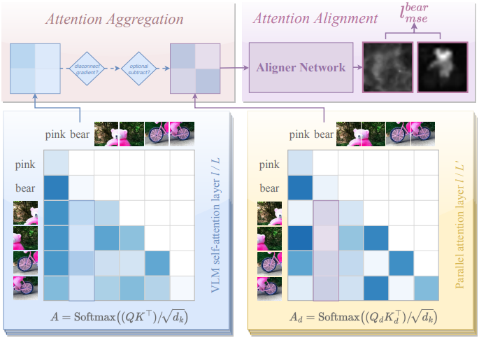
3. Aligner Network
저자들은 VLM과 DM 간의 attention 정렬을 개선하기 위해 가벼운 Aligner 네트워크를 도입했다. 이 네트워크는 병렬 또는 집계된 attention $A_d$를 단일 채널 맵으로 정제하여 DM의 attention과 직접 비교할 수 있도록 한다. Squeeze-and-Excitation network에서 영감을 받은 이 네트워크는 주요 semantic 정보를 보존하면서 attention 표현을 효율적으로 변환한다.
Aligner 네트워크는 MLP 또는 convolution을 사용하는 3~5개의 작은 layer로 구성된다. 먼저, 더 풍부한 feature를 포착하기 위해 표현을 확장하고, 비선형 변환을 적용한 다음, 이를 다시 단일 채널 attention map으로 압축한다. 경험적으로 convolution layer가 MLP보다 로컬 공간 단서를 더 잘 포착했다. Fine-tuning 과정에서 Aligner 출력은 다음과 같이 DM의 attention과 비교된다.
\[\begin{equation} L_\textrm{att} (\theta^\prime) = \sum_i \| \textrm{Aligner} (A_d^{(i)}) - p_\textrm{DM} (a \vert x^{(i)}, y^{(i)}; \theta_D) \|^2 \end{equation}\]VLM의 attention을 DM의 보다 집중된 분포로 유도하여 원래 사전 학습된 파라미터를 보존하면서 복잡한 semantic 상관관계를 포착한다.
4. Lavender Integration
Cross-Attention
전용 cross-attention layer를 가진 VLM의 경우, 각 head는 텍스트 토큰 $T_t$를 이미지 패치 $T_p$에 매핑하는 단어-패치 가중치 \(w_{(t,p)}^{hl}\)를 생성한다. 이러한 가중치를 공간 그리드로 재구성하고 head/layer 전체에 걸쳐 집계한 후, Aligner 네트워크를 적용하여 DM attention과 유사한 최종 단어별 saliency map을 생성할 수 있다. 일관성을 보장하기 위해 추출된 attention 가중치를 다음과 같이 처리한다.
- Attention 가중치를 interpolation하여 대략적인 정사각 행렬을 형성한다.
- 이미지가 여러 타일로 표현된 경우 타일을 일관된 공간 레이아웃으로 배열한다
- 후처리를 위해 map의 크기를 표준 해상도(ex. 32$\times$32)로 조정한다.
Self-Attention Only
텍스트와 이미지 패치가 단일 시퀀스에 인터리빙될 때, 토큰은 양방향 또는 인과적으로(causal) 서로에게 attention된다. 단어-패치 상관관계를 추출하려면 다음을 수행해야 한다.
- 텍스트에 해당하는 토큰 부분집합과 이미지 패치에 해당하는 토큰 부분집합을 식별한다.
- 관련 없는 attention 연결을 제외하기 위해 causal mask 또는 양방향 마스크를 적용한다.
- 추출된 attention 가중치를 재구성하고 interpolation하여 의미 있는 공간 표현을 재구성한다.
이 과정에는 적절한 텍스트 및 비주얼 토큰 인덱스를 선택하고, attention map을 정사각형 그리드로 interpolation하고, 고정 해상도(ex. 32$\times$32)로 크기를 조정하고, 선택적으로 Aligner 네트워크 출력 $A_d$ 또는 병합된 attention map을 통합하는 작업이 포함된다.
이 절차를 따라 self-attention에만 의존하는 모델에서도 비전-텍스트 정렬을 개선할 수 있도록 한다.
Experiments
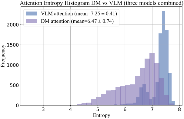
1. Empirical Verification
다음은 VLM과 DM의 attention entropy를 비교한 결과이다.
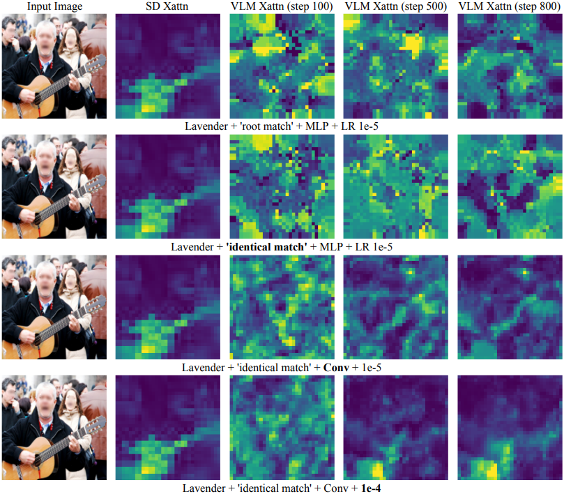
다음은 VLM과 DM의 attention을 시각적으로 비교한 결과이다. (“guitar”)
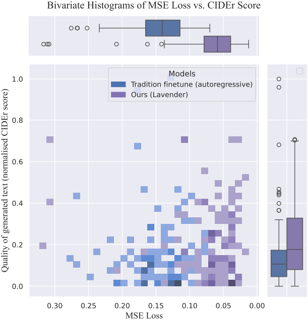
다음은 Lavender의 텍스트 생성 품질을 autoregressive fine-tuning과 비교한 결과이다.
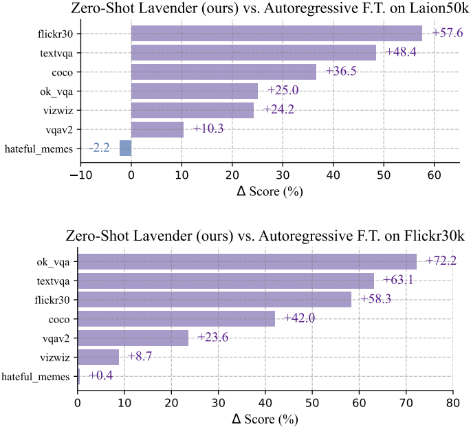
다음은 7개의 zero-shot 벤치마크에서 Lavender를 autoregressive fine-tuning과 비교한 결과이다.
2. Scaled Results with Lavender
다음은 16개의 VLM 벤치마크에 대한 zero-shot 정확도를 비교한 표이다.
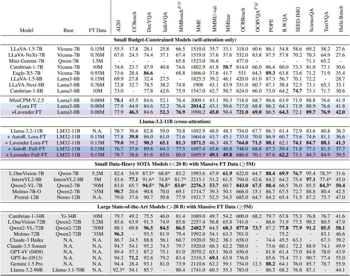
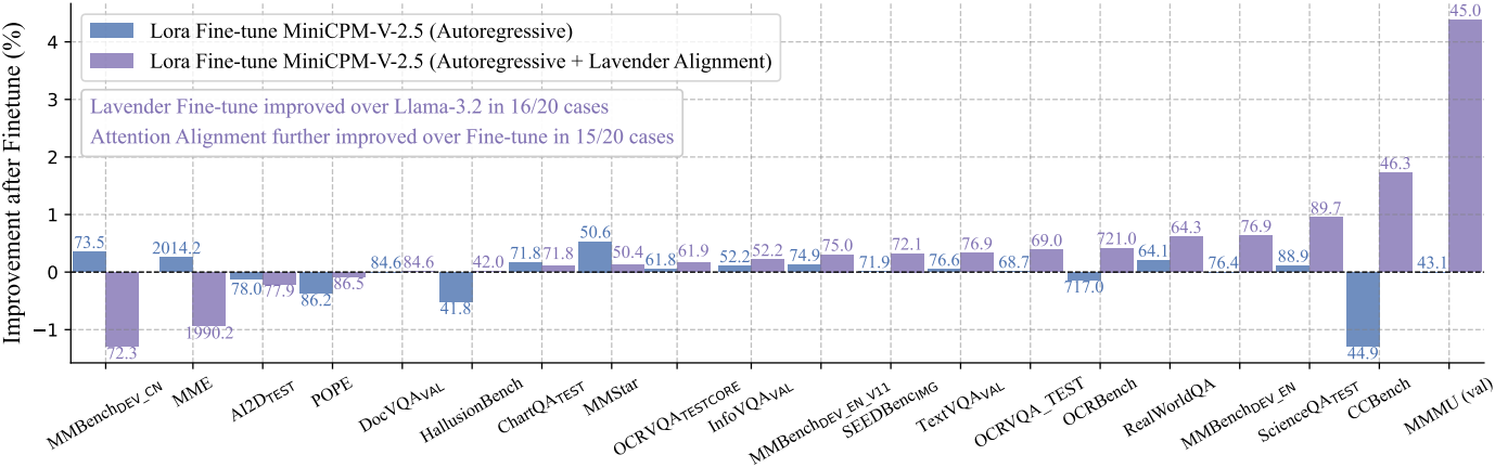
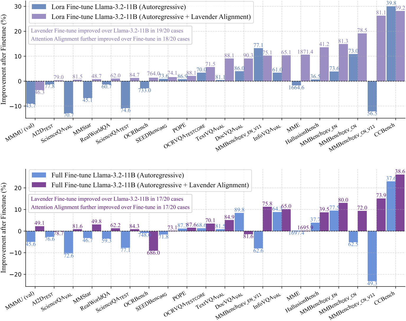
다음은 MiniCPM-Llama3-V-2.5에 대한 fine-tuning 결과이다.
다음은 Llama-3.2-11B에 대한 fine-tuning 결과이다.
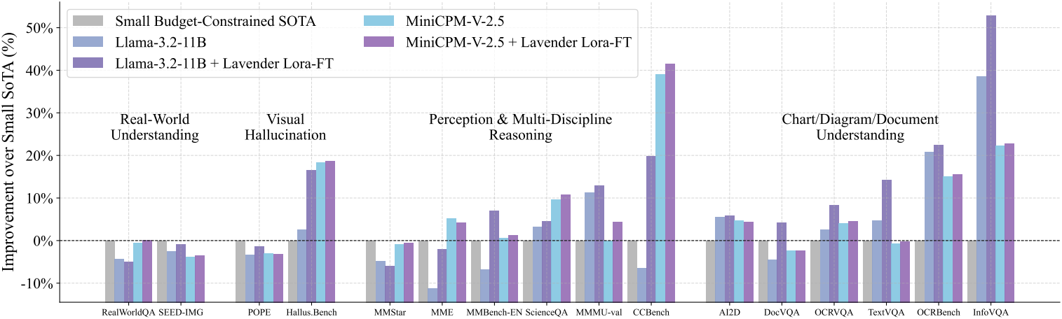
다음은 Small Budget-Constrained SOTA와의 비교 결과이다.
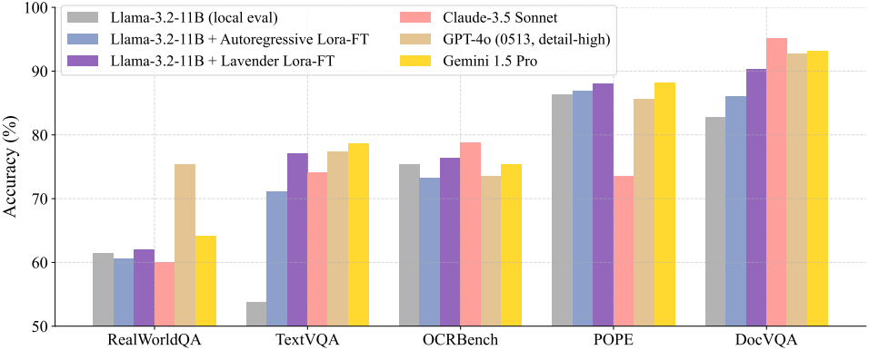
다음은 SOTA 모델과의 비교 결과이다.
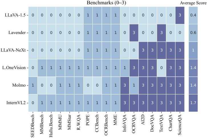
3. Data Overlapping Analysis
다음은 fine-tuning 데이터와 벤치마크 데이터 사이의 중복 정도를 비교한 결과이다. (0은 중복 없음, 1은 동일한 소스 혹은 웹 크롤링한 이미지, 3은 명시적으로 중복된 데이터)
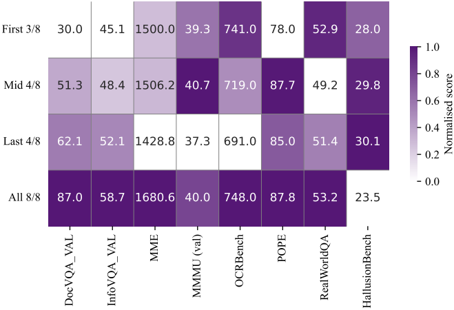
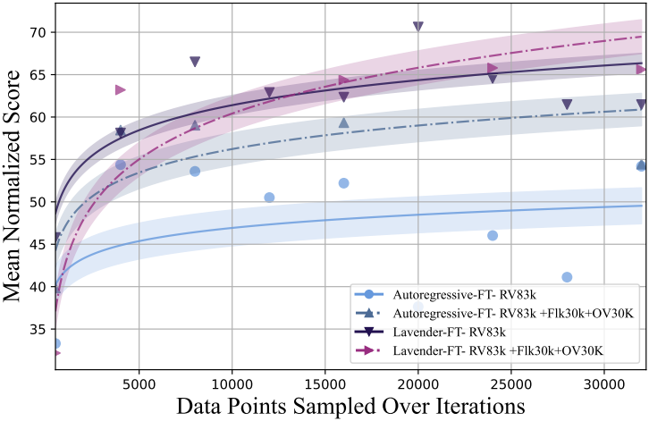
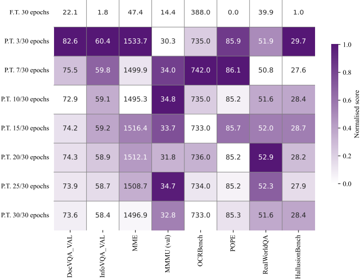
4. Scaling Behaviour
다음은 scaling 성능을 비교한 것이다. Lavender는 scaling이 더 잘되며, autoregressive fine-tuning에 비해 overfitting이 완화된다.
5. Severely Out-of-Distribution Medical Benchmark
다음은 WorldMedQA 벤치마크에 대한 OOD 성능을 비교한 결과이다.
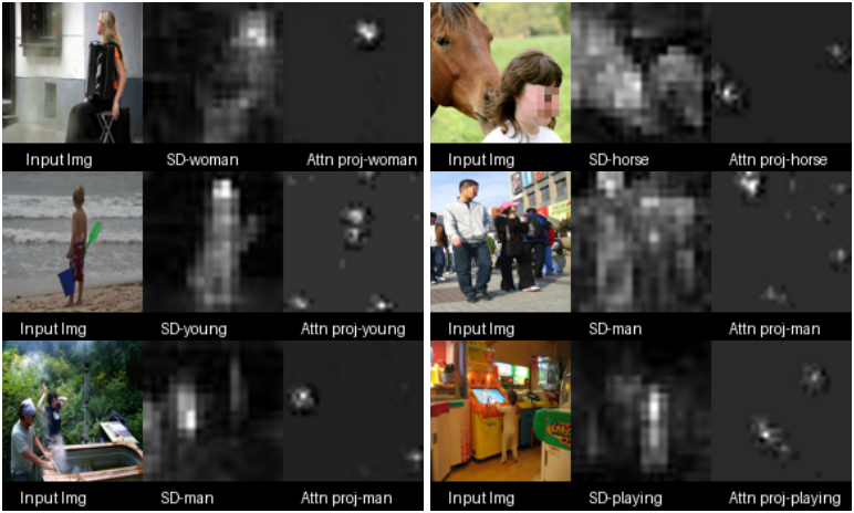
6. Qualitative Results with Llama 3.2-11B
다음은 단어별 VLM attention map을 Stable Diffusion의 attention map과 비교한 예시이다.
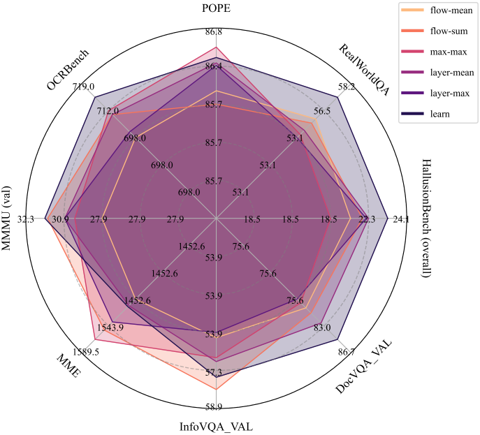
7. Ablation
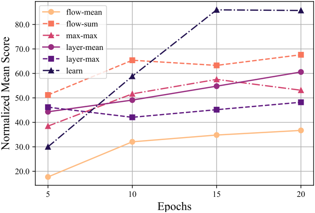
다음은 attention 집계 방법에 대한 ablation 결과이다.
다음은 Aligner 네트워크에 대한 ablation 결과이다.
다음은 layer 선택에 대한 ablation 결과이다.