[논문리뷰] EGC: Image Generation and Classification via a Diffusion Energy-Based Model
ICCV 2023. [Paper] [Page] [Github]
Qiushan Guo, Chuofan Ma, Yi Jiang, Zehuan Yuan, Yizhou Yu, Ping Luo
The University of Hong Kong | ByteDance Inc.
4 Apr 2023
Introduction
이미지 분류 및 생성은 딥 러닝 모델의 개발과 함께 상당한 발전을 보인 컴퓨터 비전의 두 가지 기본 task이다. 그러나 한 task에서 잘 수행되는 많은 SOTA 접근 방식이 다른 task에서는 성능이 좋지 않거나 다른 작업에는 적합하지 않은 경우가 많다. 두 task는 이미지 분류 task가 조건부 확률 분포 $p(y \vert x)$로 해석되고 이미지 생성 task가 알려지고 샘플링하기 쉬운 확률 분포 $p(z)$의 변환인 확률론적 관점에서 타겟 분포 $p(x)$로 공식화될 수 있다.
확률 모델의 매력적인 클래스인 EBM(Energy-Based Model)은 복잡한 확률 분포를 명시적으로 모델링하고 unsupervised 방식으로 학습할 수 있다. 또한 표준 이미지 분류 모델과 일부 이미지 생성 모델은 EBM으로 재해석할 수 있다. EBM의 관점에서 표준 이미지 분류 모델은 새로운 이미지 생성을 안내하기 위해 입력의 기울기를 활용하여 이미지 생성 모델로 용도를 변경할 수 있다.
바람직한 속성에도 불구하고 EBM은 정확한 likelihood를 계산하고 이러한 모델에서 정확한 샘플을 합성하는 난해성으로 인해 학습에 어려움을 겪고 있다. 임의의 energy model은 기울기의 급격한 변화를 나타내어 Langevin 동역학으로 샘플링을 불안정하게 만든다. 이 문제를 개선하기 위해 spectral normalization은 일반적으로 energy model의 Lipschitz 상수를 제한하기 위해 채택된다. 이 normalization을 사용하더라도 실제 데이터의 확률 분포가 일반적으로 고차원 space에서 선명하여 낮은 데이터 밀도 영역에서 이미지 샘플링에 대한 부정확한 guidance를 제공하기 때문에 EBM에서 생성된 샘플은 여전히 충분히 경쟁력이 없다.
Diffusion model은 GAN에 비해 경쟁력 있고 심지어 우수한 이미지 생성 성능을 입증했다. Diffusion model에서는 학습을 위한 diffusion process를 통해 이미지에 Gaussian noise를 추가하고, reverse process를 학습하여 가우시안 분포를 다시 데이터 분포로 변환한다. Noise가 추가된 데이터 포인트는 낮은 데이터 밀도 영역을 채워 추정 score의 정확도를 향상시켜 안정적인 학습 및 이미지 샘플링을 제공한다.
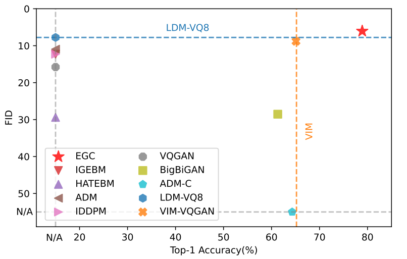
보 논문은 EBM의 유연성과 diffusion model의 안정성에 동기 부여되여 단일 신경망을 사용하여 이미지 분류 및 생성 task 모두에서 우수한 성능을 달성하는 새로운 energy-based classifier and generator, 즉 EGC를 제안한다. EGC는 forward pass에서는 classifier고 backward pass에서는 이미지 generator이다. 이미지가 주어진 레이블의 조건 분포 $p(y \vert x)$를 예측하는 기존 classifier와 달리 EGC의 forward pass는 소스 이미지가 주어진 노이즈 이미지와 레이블의 결합 분포 $p(x, y)$를 모델링한다. 레이블 $y$를 주변화(marginalizing)함으로써 noisy한 이미지의 로그 확률 기울기, 즉 unconditional score를 사용하여 noise에서 이미지를 복원한다. 분류 확률 $p(y \vert x)$는 한 단계 backward pass 내에서 unconditional score와 함께 classifier guidance를 제공한다.
Method
Overview
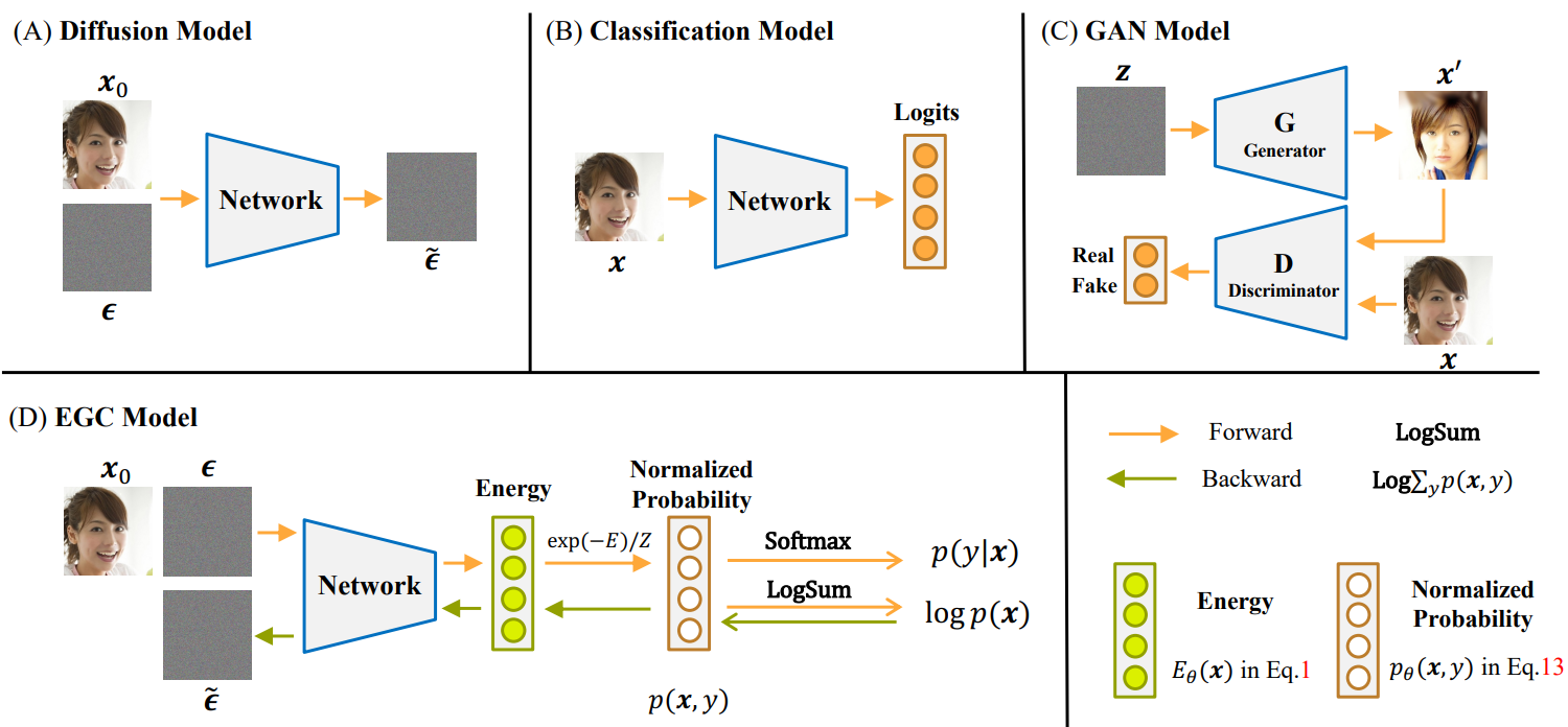
위 그림에서 볼 수 있듯이 EGC 모델은 forward pass 동안 energy를 추정하여 결합 분포 $p(x, y)$를 모델링하는 classifier로 구성된다. 조건부 확률 $p(y \vert x)$는 Softmax 함수에 의해 생성된다. 네트워크의 backward pass는 unconditional score $\nabla_x \log p(x)$와 class guidance $\nabla_x \log p(y \vert x)$를 $y$를 marginalizing하여 모두 단일 step으로 생성한다. 낮은 데이터 밀도 영역을 채우기 위해 diffusion process를 채택하고 정규화된 확률 밀도의 직접적인 최적화를 우회하는 Fisher divergence를 사용하여 unconditional score를 최적화한다.
Background
EBM은
\[\begin{equation} p_\theta (x) = \frac{\exp (-E_\theta (x))}{Z (\theta)} \\ \textrm{where} \quad Z(\theta) = \int \exp (-E_\theta (x)) dx \end{equation}\]로 정의되어 임의의 확률 밀도 함수 $p_\textrm{data} (x)$를 $x \in \mathbb{R}^D$에서 근사한다. 여기서 $E_\theta (x) : \mathbb{R}^D \rightarrow \mathbb{R}$는 energy function이라 부르며 각 데이터 포인트를 스칼라로 매핑한다. $Z(\theta)$는 확률의 전체 합을 1로 만들기 위한 partition function으로, 고차원의 $x$에 대하여 수치적으로 다룰 수 없다. 일반적으로 신경망 $f_\theta (x) = −E_\theta (x)$를 사용하여 energy function을 parameterize할 수 있다. 독립적인 데이터에서 확률 모델을 학습하기 위한 사실상의 표준은 maximum likelihood estimation이다. Log-likelihood function은 다음과 같다.
\[\begin{equation} \mathcal{L} (\theta) = \mathbb{E}_{x \sim p_\textrm{data} (x)} [\log p_\theta (x)] \simeq \frac{1}{N} \sum_{i=1}^N \log p_\theta (x_i) \end{equation}\]여기서 $N$개의 샘플 $x_i \sim p_\textrm{data} (x)$를 관찰한다. EBM의 로그 확률 기울기는 다음 두 항으로 구성된다.
\[\begin{equation} \frac{\partial \log p_\theta (x)}{\partial \theta} = \frac{\partial f_\theta (x)}{\partial \theta} - \mathbb{E}_{x' \sim p_\theta (x')} [\frac{\partial f_\theta (x')}{\partial \theta}] \end{equation}\]두 번째 항은 Markov Chain Monte Carlo (MCMC)를 사용하여 모델 분포 $p_\theta (x’)$에서 합성된 샘플로 근사화할 수 있다. Langevin MCMC는 먼저 간단한 prior 분포에서 초기 샘플을 추출하고 다음과 같이 공식화할 수 있는 모드에 도달할 때까지 샘플을 반복적으로 업데이트한다.
\[\begin{equation} x_{i+1} \leftarrow x_i + c \nabla_x \log p(x_i) + \sqrt{2c} \epsilon_i \end{equation}\]여기서 $x_0$는 prior 분포(ex. 가우시안 분포)에서 랜덤하게 샘플링되고 $\epsilon_i \sim \mathcal{N} (0, I)$이다. 그러나 고차원 분포의 경우 MCMC를 실행하여 수렴된 샘플을 생성하는 데 시간이 오래 걸린다.
1. Energy-Based Model with Diffusion Process
Diffusion model은 Markov chain으로 공식화할 수 있는 forward process 중에 소스 샘플에 noise를 점진적으로 주입한다.
\[\begin{equation} q(x_{1:T} \vert x_0) = \prod_{t=1}^T q(x_t \vert x_{t-1}), \\ q(x_t \vert x_{t-1}) = \mathcal{N} (x_t; \sqrt{\vphantom{1} \alpha_t} x_{t-1}, \beta_t I) \end{equation}\]여기서 $x_0$은 소스 샘플을 나타내고 $\alpha_t = 1 − \beta_t$를 나타낸다. 임의의 timestep $t$에 대해 반복 샘플링 없이 다음 가우시안 분포에서 직접 샘플링할 수 있다.
\[\begin{equation} q(x_t \vert x_0) = \mathcal{N}(x_t; \sqrt{\vphantom{1} \bar{\alpha}_t} x_0, (1 - \bar{\alpha}_t) I) \end{equation}\]베이즈 정리에 따라 posterior $q(x_{t-1} \vert x_t, x_0)$에 의해 forward process를 reverse시킬 수 있다.
\[\begin{equation} q(x_{t-1} \vert x_t, x_0) = \mathcal{N} (x_{t-1}; \tilde{\mu} (x_t, x_0), \tilde{\beta}_t I) \\ \tilde{\mu} (x_t, x_0) = \frac{\sqrt{\vphantom{1} \bar{\alpha}_{t-1}} \beta_t}{1 - \bar{\alpha}_t} x_0 + \frac{\sqrt{\alpha_t} (1 - \bar{\alpha}_{t-1})}{1 - \bar{\alpha}_t} x_t \\ \tilde{\beta}_t = \frac{1 - \bar{\alpha}_{t-1}}{1 - \bar{\alpha}_t} \beta_t \end{equation}\]$x_0$는 reverse process에서 알 수 없으므로
\[\begin{equation} p_\theta (x_{t-1} \vert x_t) = q(x_{t-1} \vert x_t, x_0 = \mu_\theta (x_t)) \end{equation}\]로 posterior를 근사하여 관찰된 샘플 $x_t$를 denoise한다.
Tweedie’s Formula에 따르면, 확률 변수 $z \sim \mathcal{N} (z; \mu_z, \Sigma_z)$가 주어지면 다음과 같이 가우시안 분포의 평균을 추정할 수 있다.
\[\begin{equation} \mathbb{E}[\mu_z \vert z] = z + \Sigma_z \nabla_z \log p(z) \end{equation}\]Tweedie’s Formula를 $q(x_t \vert x_0)$ 식에 적용하면 $x_t$의 평균에 대한 추정치를 다음과 같이 나타낼 수 있다.
\[\begin{equation} \sqrt{\vphantom{1} \bar{\alpha}_t} x_0 = x_t + (1 - \bar{\alpha}_t) \nabla_{x_t} \log q(x_t \vert x_0) \end{equation}\]$x_t$는
\[\begin{equation} x_t = \sqrt{\vphantom{1} \bar{\alpha}_t} x_0 + \sqrt{1 - \bar{\alpha}_t} \epsilon \end{equation}\]로 분해되기 때문에 score function은 다음과 같다.
\[\begin{equation} \nabla_{x_t} \log q(x_t \vert x_0) = - \frac{\epsilon_t}{\sqrt{1 - \bar{\alpha}_t}} \end{equation}\]EBM $p_\theta (x_t)$로 확률 밀도 함수 $q(x_t \vert x_0)$를 근사하고 $q(x_t \vert x_0)$와 $p_\theta (x_t)$ 사이의 Fisher divergence를 최소화하여 파라미터를 최적화한다.
\[\begin{equation} \mathcal{D}_F = \mathbb{E}_q [\frac{1}{2} \| \nabla_{x_t} \log q(x_t \vert x_0) - \nabla_{x_t} \log p_\theta (x_t) \|^2] \end{equation}\]EBM의 경우 $\nabla_x \log p_\theta (x) = \nabla_x f_\theta (x)$로 score를 쉽게 얻을 수 있다. EBM의 로그 확률을 직접 최적화하는 것과 비교하여 Fisher divergence는 $Z(\theta)$로 parameterize된 정규화된 밀도를 최적화하고 목표 score를 $\nabla_{x_t} \log q(x_t \vert x_0)$로 가우시안 분포에서 직접 샘플링할 수 있다.
EGC
EBM은 discriminative model과 본질적으로 연결되어 있다. $C$개의 클래스에 대한 classification 문제의 경우 discriminative classifier는 데이터 샘플 $x \in \mathbb{R}^D$를 길이 $C$의 logit 벡터에 매핑한다. $y$번째 레이블의 확률은 Softmax 함수를 사용하여 표시된다.
\[\begin{equation} p(y \vert x) = \frac{\exp (f(x)[y])}{\sum_{y'} \exp(f(x)[y'])} \end{equation}\]여기서 $f(x)[y]$는 $y$번째 logit이다. 베이즈 정리를 사용하여 판별 조건부 확률은
\[\begin{equation} p(y \vert x) = \frac{p(x, y)}{\sum_{y'} p(x, y')} \end{equation}\]로 표현될 수 있다. 데이터 샘플 $x$와 레이블 $y$의 결합 확률은 다음과 같이 모델링할 수 있다.
\[\begin{equation} p_\theta (x, y) = \frac{\exp (f_\theta (x) [y])}{Z(\theta)} \end{equation}\]y를 marginalizing하여 데이터 샘플 $x$의 score를 다음과 같이 구한다.
\[\begin{equation} \nabla_x \log p(x) = \nabla_x \log \sum_y \exp (f_\theta (x)[y]) \end{equation}\]일반적인 classifier와 달리 free energy function $E_\theta (x) = −\log \sum_y exp(f_\theta (x)[y])$도 샘플 생성에 최적화되어 있다.
강력한 판별 성능과 생성 성능을 모두 달성하기 위해 energy-based classifier를 diffusion process와 통합할 것을 제안한다. 특히 energy-based classifier $p_\theta (x_t, y)$를 사용하여 조건부 확률 밀도 함수 $q(x_t, y \vert x_0)$를 근사화한다. EBM에 대한 Fisher divergence의 최적화로 인해 log-likelihood를 다음과 같이 분해한다.
\[\begin{equation} \log p_\theta (x_t, y) = \log p_\theta (x_t) + \log p_\theta (y \vert x_t) \end{equation}\]Score $\nabla_{x_t} \log p_\theta (x_t)$는 Fisher divergence를 최소화하여 최적화된다. 조건부 확률 $p_\theta (y \vert x_t)$에 대해서는 표준 cross-entropy loss를 채택하여 최적화한다.
Energy-based classifier를 diffusion process와 통합하는 이점 중 하나는 classifier가 컨디셔닝 정보 $y$를 통해 생성하는 데이터를 명시적으로 제어하기 위한 guidance를 제공한다는 것이다. 베이즈 정리에 따라 조건부 score는 다음과 같이 도출할 수 있다.
\[\begin{equation} \nabla \log p_\theta (x_t \vert y) = \nabla \log p_\theta (x_t) + \nabla \log p_\theta (y \vert x_t) \end{equation}\]결합 확률 $p_\theta (x_t, y)$는 신경망으로 parameterize된다. 그리고 EGC 모델의 forward pass는 조건부 확률 $p_\theta (y \vert x)$를 예측하는 discriminative model인 반면, 신경망의 backward pass는 score를 예측하는 생성 모델이고 점진적으로 데이터를 denoise하기 위한 classifier guidance이다.
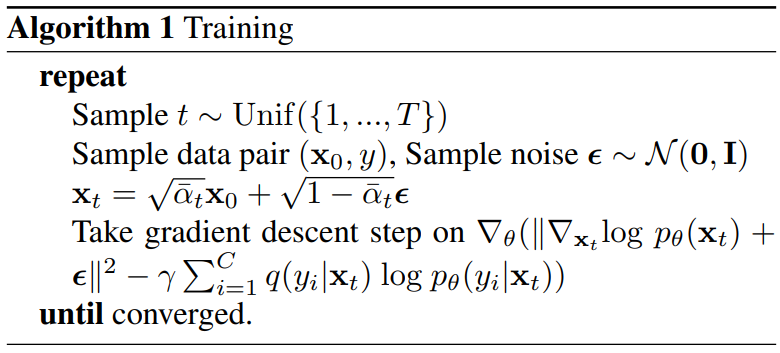
EGC 모델의 전체적인 학습 loss는 다음과 같다.
\[\begin{aligned} \mathcal{L} = \;& \mathbb{E}_q [\frac{1}{2} \| \nabla_{x_t} \log q(x_t \vert x_0) - \nabla_{x_t} \log p_\theta (x_t) \|^2 \\ & - \sum_{i=1}^C q(y_i \vert x_t, x_0) \log p_\theta (y_i \vert x_t)] \end{aligned}\]여기서 첫 번째 항은 noisy한 샘플 $x_t$에 대한 reconstruction loss이고 두 번째 항은 denoising process가 주어진 레이블과 일치하는 샘플을 생성하도록 하는 classification loss이다. 학습 절차는 신경망의 안정적인 최적화를 보장하기 위해 noise를 타겟 score로 채택하며, Algorithm 1과 같다. 또한 hyperparameter $\gamma$가 도입되어 두 loss 항의 균형을 맞춘다.
Experiments
- 데이터셋
- Conditional: CIFAR-10, CIFAR-100, ImageNet
- Unconditional: CelebA-HQ, LSUN Church
- Details
1. Hybrid Modeling
EGC model
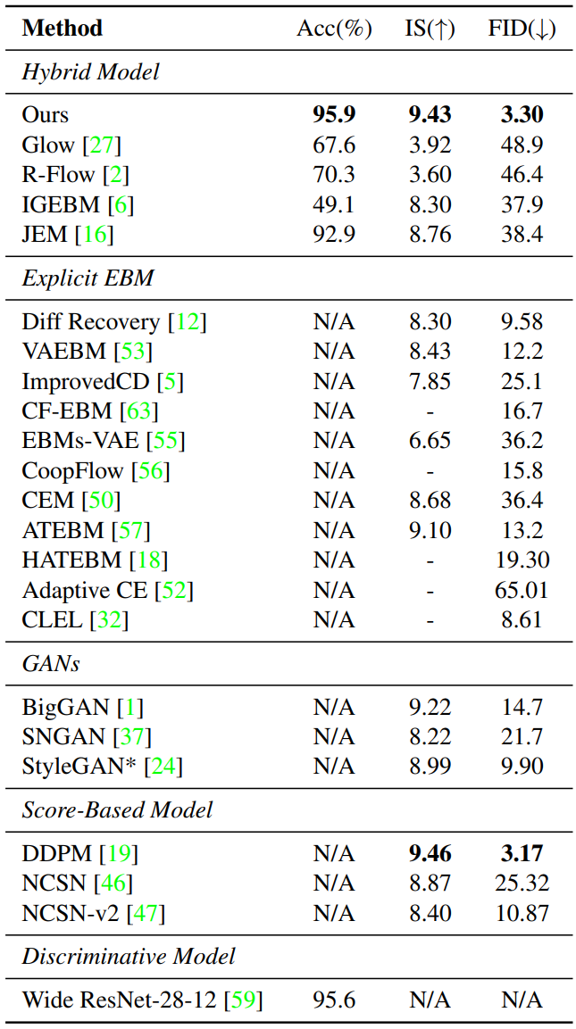
다음은 CIFAR-10에서의 결과이다.
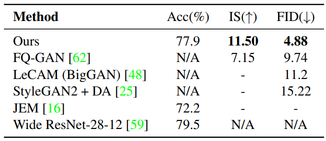
다음은 CIFAR-100에서의 결과이다.
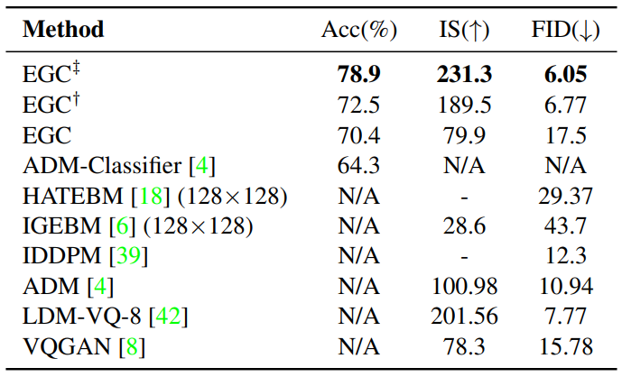
다음은 ImageNet-1k 256$\times$256에서의 결과이다. $\dagger$는 conditional model과 unconditional model을 공동으로 학습한 모델이고, $\ddagger$는 RandResizeCrop을 통합한 모델이다.
Unsupervised EGC model
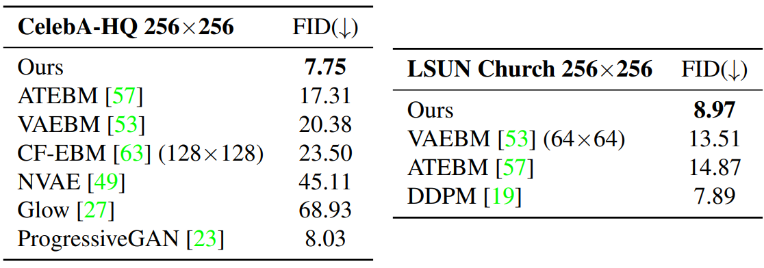
다음은 CelebA-HQ와 LSUN-Church에서 다른 EBM들과 비교한 표이다.
Ablation study
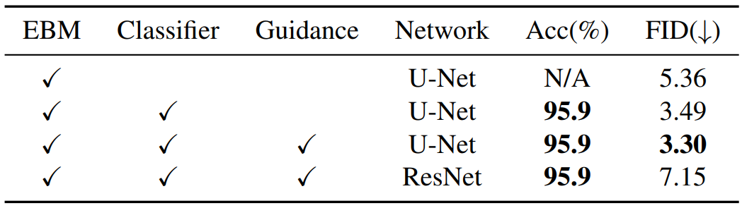
다음은 CIFAR-10에서의 ablation study 결과이다.
2. Application and Analysis
Interpolation
다음은 두 생성된 샘플을 interpolate한 결과이다. $x_T$와 $x_0$는 각각 noise 샘플과 생성된 샘플을 interpolate한 것이다.
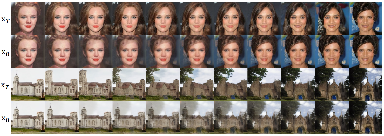
Image inpainting
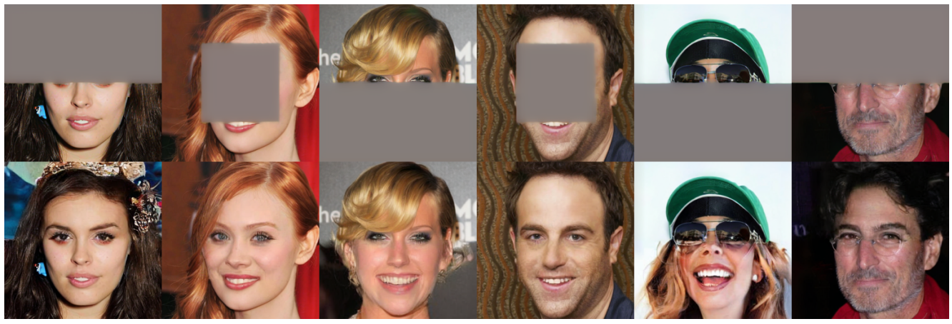
다음은 CelebA-HQ 256$\times$256에서 inpainting 결과이다.
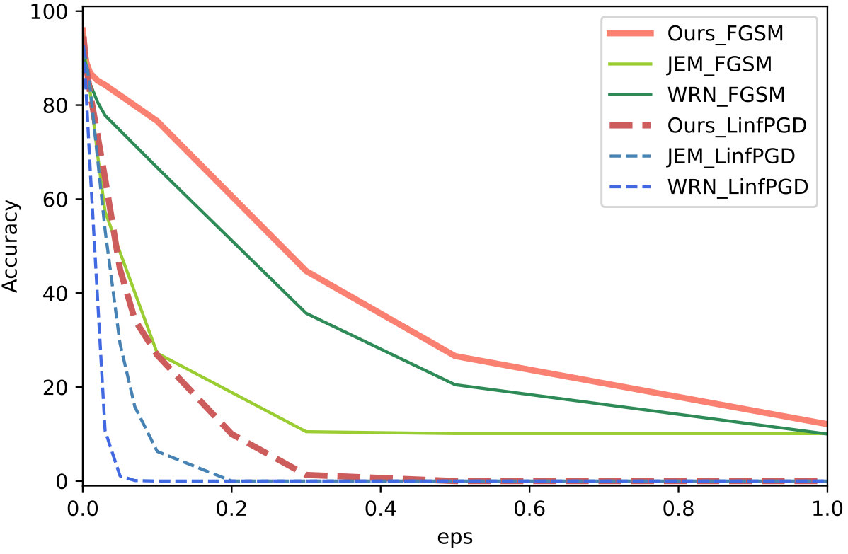
Robustness
다음은 CIFAR-10에서 adversarial attack (PGC, FGSM)에 대한 robustness 평가한 그래프이다.
Visualize Energy
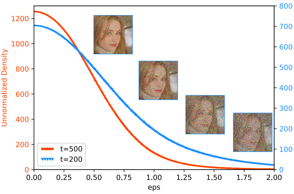
다음은 $x_t$의 unnormalized probability density이다. x축은 $x_t$의 noise level로, 각 timestep에서 noise 값의 평균이다.
다음은 $t = 500$(왼쪽)과 $t = 200$(오른쪽)에서의 샘플에 대한 unnormalized probability density이다. 직교하는 두 noise를 선택하고 둘의 선형 결합을 plot한 것이다.
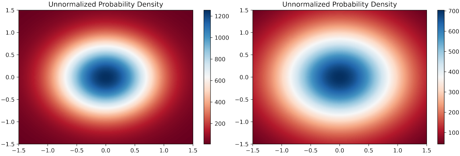
확률 밀도가 가우시안 분포와 비슷한 모양을 보인다는 것을 확인할 수 있다.
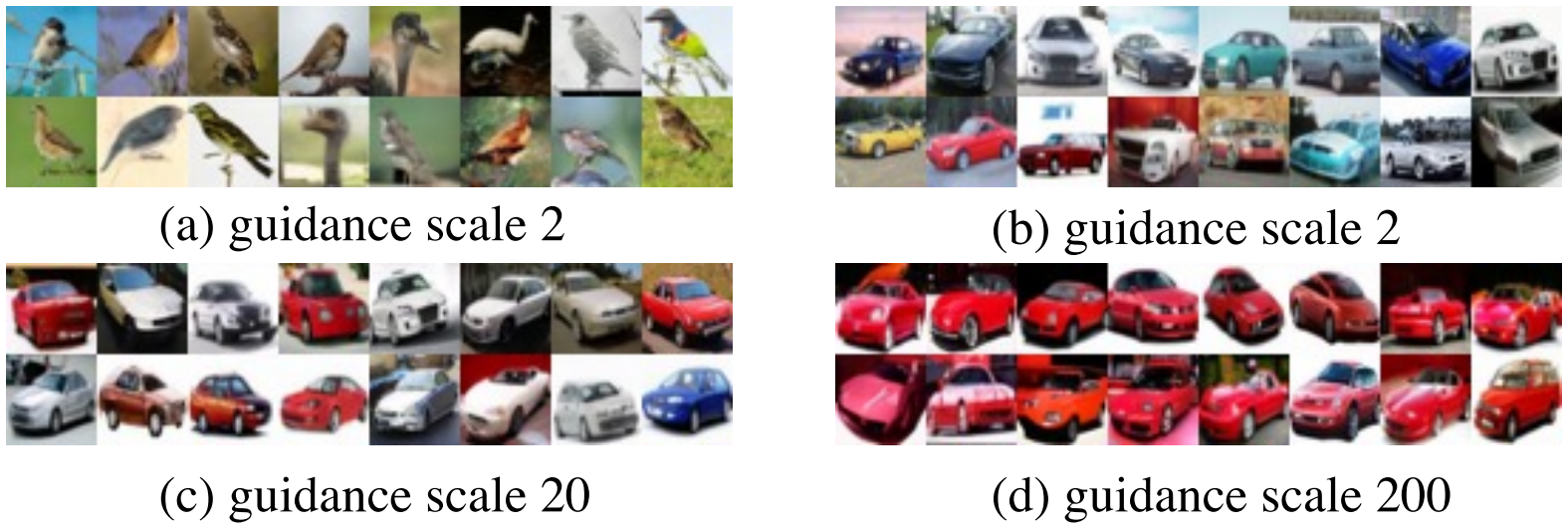
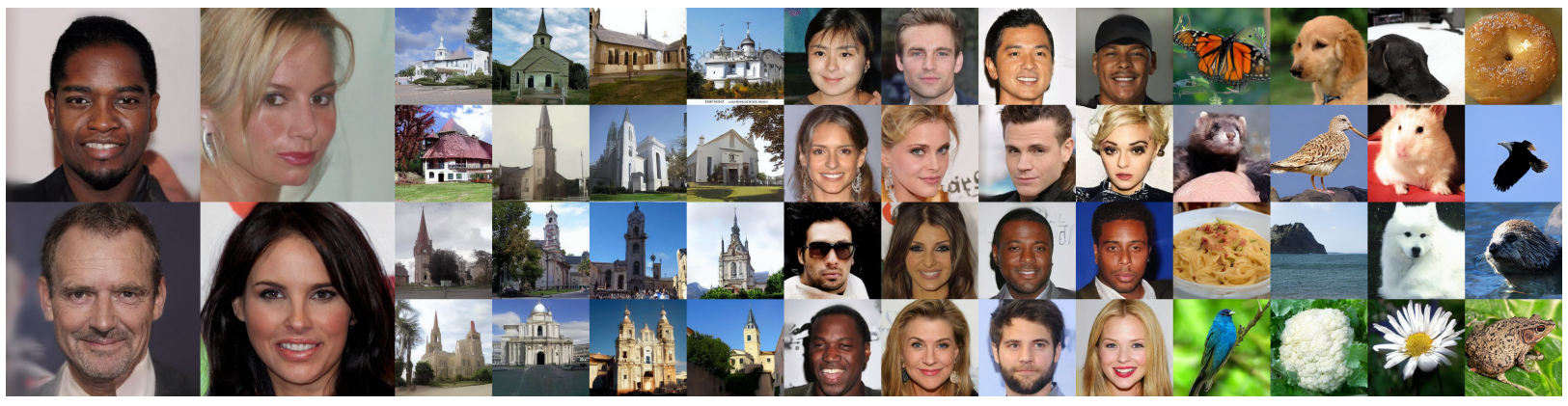
Conditional sampling
다음은 조건부 샘플링 결과이다.