[논문리뷰] Conditional Image Generation with Score-Based Diffusion Models (CMDE)
arXiv 2021. [Paper]
Georgios Batzolis, Jan Stanczuk, Carola-Bibiane Schönlieb, Christian Etmann
University of Cambridge | Deep Render
26 Nov 2021

Introduction
Score 기반 diffusion model은 이미지 생성 및 likelihood 추정 모두에서 state-of-the-art 성능을 달성하는 것 외에도 학습 불안정 또는 mode collapse로 인해 어려움을 겪지 않는다. 또한 고해상도에서의 시간 복잡도는 autoregressive 모델보다 훨씬 낫다. 따라서 score 기반 diffusion model은 심층 생성 모델링에 매우 매력적인 모델이다.
본 논문에서는 score 기반 diffusion model을 조건부 이미지 생성에 어떻게 적용할 수 있는지 살펴본다. 조건부 score를 추정하는 가장 좋은 방법을 찾기 위해 기존 접근법의 검토 및 분류를 수행하고 체계적 비교를 수행한다. 정당한 이유 없이 사용된 conditional denoising estimator에 대한 타당성을 증명함으로써 향후 연구에서 이를 사용할 수 있는 확고한 이론적 기반을 제공한다. 또한 입력 텐서의 서로 다른 부분이 서로 다른 속도에 따라 diffuse되는 multi-speed diffusion을 지원하도록 원래 프레임워크를 확장한다. 이를 통해 조건부 score의 새로운 estimator를 도입하고 추가 연구를 위한 길을 열 수 있다.
Methods
1. Background: Score matching through Stochastic Differential Equations
1.1 Unconditional generation
최근 연구에서 score 기반 생성 모델과 diffusion 기반 생성 모델은 SDE에 의해 구동되는 diffusion을 통해 하나의 연속 시간 score 기반 프레임워크로 통합되었다. Forward diffusion process
\[\begin{equation} dx = \mu (x, t) dt + \sigma (t) dw \end{equation}\]는 다음 SDE에 의해 제어되는 reverse diffusion process를 갖는다.
\[\begin{equation} dx = [\mu (x, t) - \sigma (t)^2 \nabla_x \ln p_{X_t} (x)] dt + \sigma (t) d \bar{w} \end{equation}\]$\bar{w}$는 표준 Wiener process이다.
Forward diffusion process는 target distribution $p(x_0)$를 diffused distribution $p(x_T)$로 변환한다. Forward SDE의 drift와 diffusion 계수를 적절하게 선택함으로써 충분히 긴 시간 $T$ 후에 diffusio 분포 $p(x_T)$가 $\mathcal{N}(0,I)$과 같은 단순 분포에 가까워지는지 확인할 수 있다. 이 단순 분포 $\pi$를 prior distribution라고 한다.
모든 $t$에 대해 주변 분포의 score인 $\nabla_{x_t} \ln p(x_t)$에 접근할 수 있는 경우 reverse diffusion process를 유도하고 시뮬레이션하여 $p_T$를 $p_0$에 매핑할 수 있다. 실제로, 신경망 $s_\theta (x_t, t) \approx \nabla_{x_t} \ln p(x_t)$에 의해 시간 종속 분포의 score를 근사화하고 prior distribution $\pi ≈ p(x_T)$를 $p_\theta(x) \approx p(x_0)$으로 매핑하여 시간 $T$에서 시간 $0$까지 reverse-time SDE를 해결한다. Euler–Maruyama나 기타 이산화 전략과 같은 표준 numerical SDE solver를 사용하여 reverse SDE를 통합할 수 있다. 저자들은 표준 통합 step을 고정된 수의 Langevin MCMC step과 결합하여 각 중간 timestep에서 분포 score에 대한 지식을 활용할 것을 제안한다. MCMC correction step은 샘플링을 향상시키며, 결합된 알고리즘은 predictor-corrector 방식으로 알려져 있다.
신경망 $s_\theta (x_t, t)$를 score $\nabla_{x_t} \ln p(x_t)$로 근사하기 위하여 weighted Fisher’s divergence를 최소화한다.
\[\begin{equation} \mathcal{L}_{SM} (\theta) := \frac{1}{2} \mathbb{E}_{t \sim U(0,T), x_t \sim p(x_t)} [\lambda(t) \| \nabla_{x_t} \ln p(x_t) - s_\theta (x_t, t) \|_2^2 ] \end{equation}\]여기서 \(\lambda : [0,T] \rightarrow \mathbb{R}_{+}\)는 양의 가중치 함수이다.
Ground-truth score $\nabla_{x_t} \ln p(x_t)$를 모르기 때문에 직접 위 식으로 최적화를 할 수 없다, 따라서, 실제로는 $\theta$에 의존하지 않는 추가 항을 더한 다른 목적 함수를 사용한다.
\[\begin{equation} \mathcal{L}_{DSM} (\theta) := \frac{1}{2} \mathbb{E}_{t \sim U(0,T), x_0 \sim p(x_0), x_t \sim p(x_t \vert x_0)} [\lambda(t) \| \nabla_{x_t} \ln p(x_t \vert x_0) - s_\theta (x_t, t) \|_2^2 ] \end{equation}\]$\nabla_{x_t} \ln p(x_t \vert x_0)$는 수치적으로 계산할 수 있다. 기대값은 다음과 같은 Monte Carlo 추정을 사용한다.
- $[0, T]$애서 uniform distribution으로 $t$를 샘플링한다.
- $\tilde{x}$를 target distribution $p_0$에서 샘플링한다.
- 각 $\tilde{x}$에 대하여 $x_t$를 샘플링한다. (forward process)
- 모든 샘플에 대한 기대값을 계산한다.
2. Conditional generation
연속적인 score-matching 프레임워크는 조건부 생성으로 확장할 수 있다. 타겟 이미지 $x$와 컨디션 이미지 $y$에 대하여 $p(x \vert y)$를 구해야 한다. Forward diffusion process로 diffused distribution $p(x_t \vert y)$를 구한 다음 unconditional한 방법과 동일하게 reverse-time SDE를 유도할 수 있다.
\[\begin{equation} dx = [\mu (x, t) - \sigma (t)^2 \nabla_x \ln p_{X_t} (x \vert y)] dt + \sigma(t) d \bar{w} \end{equation}\]Score $\nabla_{x_t} \ln p(x_t \vert y)$를 학습하여야 reverse-time diffusion을 사용하여 샘플링할 수 있다.
본 논문에서는 다음과 같은 접근 방식들로 조건부 score를 추정하는 방식을 살펴본다.
- Conditional denoising estimators
- Conditional diffusive estimators
- Multi-speed conditional diffusive estimators (본 논문의 방법)
조건부 socre를 추정하기 위한 또다른 방법은 unconditional score model과 학습된 $p(y \vert x_t)$를 사용하는 방법으로,
\[\begin{equation} \nabla_{x_t} \ln p(x_t \vert y) = \nabla_{x_t} \ln p(x_t) + \nabla_{x_t} \ln p(y \vert x_t) \end{equation}\]을 사용하여 조건부 score를 추정한다. 다른 접근 방식들과 다르게 이 방법은 분리된 모델이 필요하다. 본 논문에서는 이러한 접근 방식을 다루지 않는다.
2.1 Conditional denoising estimator (CDE)
Conditional denoising estimator (CDE)는 denoising score matching을 사용하여 조건부 score를 추정하는 방법이다. 조건부 score를 근사하기 위하여 conditional denoising estimator가
\[\begin{equation} \frac{1}{2} \mathbb{E}_{t \sim U(0,T), x_0 \sim p(x_0), x_t \sim p(x_t \vert x_0)} [\lambda(t) \| \nabla_{x_t} \ln p(x_t \vert x_0) - s_\theta (x_t, y, t) \|_2^2 ] \end{equation}\]를 최소화한다. 이 estimator는 이전 연구들에서 성공적인 결과를 보였다.
그럼에도 불구하고 이 estimator는 위의 목적 함수를 학습하면 원하는 조건부 분포를 생성하는 이유에 대한 이론적 정당성 없이 사용되었다. $p(x_t \vert y)$는 목적 함수에 나타나지 않기 때문에 minimizer가 정확한 값에 근접하는지 명확하지 않다. 위 loss의 minimizer가 정확한 조건부 score $p(x_t \vert y)$를 근사한다는 것은 아래와 같이 증명할 수 있다.
증명)
Tower law에 의해 $$ \begin{aligned} & \mathbb{E}_{t \sim U(0,T), (x_0,y) \sim p(x_0, y), x_t \sim p(x_t \vert x_0)} [\lambda(t) \| \nabla_{x_t} \ln p(x_t \vert x_0) - s_\theta (x_t, y, t) \|_2^2 ] \\ =& \mathbb{E}_{t \sim U(0,T), y \sim p(y), x_0 \sim p(x_0 \vert y), x_t \sim p(x_t \vert x_0)} [\lambda(t) \| \nabla_{x_t} \ln p(x_t \vert x_0) - s_\theta (x_t, y, t) \|_2^2 ] \\ =& (*) \end{aligned} $$ $x_t$가 $y$에 독립이므로 $$ \begin{equation} (*) = \mathbb{E}_{t \sim U(0,T), y \sim p(y), x_0 \sim p(x_0 \vert y), x_t \sim p(x_t \vert x_0, y)} [\lambda(t) \| \nabla_{x_t} \ln p(x_t \vert x_0, y) - s_\theta (x_t, y, t) \|_2^2 ] \end{equation} $$ 이다. $y$와 $t$를 고정시키면 $$ \begin{aligned} & \mathbb{E}_{x_0 \sim p(x_0 \vert y), x_t \sim p(x_t \vert x_0, y)} [\lambda(t) \| \nabla_{x_t} \ln p(x_t \vert x_0, y) - s_\theta (x_t, y, t) \|_2^2 ] \\ =& \mathbb{E}_{x_t \sim p(x_t \vert y)} [\lambda(t) \| \nabla_{x_t} \ln p(x_t \vert y) - s_\theta (x_t, y, t) \|_2^2 ] \end{aligned} $$ 이고, $t$와 $y$가 임의적이므로 모든 $t$와 $y$에 대해 위 식이 성립하고, 대입하면 $$ \begin{equation} (*) = \mathbb{E}_{t \sim U(0,T), y \sim p(y), x_t \sim p(x_t \vert y)} [\lambda(t) \| \nabla_{x_t} \ln p(x_t \vert y) - s_\theta (x_t, y, t) \|_2^2 ] \end{equation} $$ 이다. Tower Law에 의해 $$ \begin{equation} (*) = \mathbb{E}_{t \sim U(0,T), (x_t, y) \sim p(x_t, y)} [\lambda(t) \| \nabla_{x_t} \ln p(x_t \vert y) - s_\theta (x_t, y, t) \|_2^2 ] \end{equation} $$ 이다. 즉, $$ \begin{aligned} & \mathbb{E}_{t \sim U(0,T), (x_0,y) \sim p(x_0, y), x_t \sim p(x_t \vert x_0)} [\lambda(t) \| \nabla_{x_t} \ln p(x_t \vert x_0) - s_\theta (x_t, y, t) \|_2^2 ] \\ =& \mathbb{E}_{t \sim U(0,T), (x_t, y) \sim p(x_t, y)} [\lambda(t) \| \nabla_{x_t} \ln p(x_t \vert y) - s_\theta (x_t, y, t) \|_2^2 ] \end{aligned} $$
2.2 Conditional diffusive estimator (CDiffE)
Conditional diffusive estimators (CDiffE)의 핵십 아이디어는 $p(x_t \vert y)$를 바로 학습하는 대신 $x$와 $y$ 모두 diffuse하여 $p(x_t \vert y_t)$로 근사하는 것이다. $\nabla_{x_t} \ln p(x_t \vert y_t)$를 학습하는 것이 최적화를 쉽게 만들며 바로 $\nabla_{x_t} \ln p(x_t \vert y)$를 학습하는 것보다 결과가 좋다.
$z_t := (x_t, y_t)$이고 $n_x$를 $x$의 차원이라 두면
\[\begin{equation} \nabla_{x_t} \ln p(x_t \vert y_t) = \nabla_{x_t} \ln p(x_t, y_t) = \nabla_{z_t} \ln p(z_t) [: n_x] \end{equation}\]이므로, unconditional한 경우와 비슷한 목적함수를 사용할 수 있다.
\[\begin{equation} \frac{1}{2} \mathbb{E}_{t \sim U(0,T), z_0 \sim p_0 (z_0), z_t \sim p(z_t \vert z_0)} [\lambda(t) \| \nabla_{z_t} \ln p(z_t \vert z_0) - s_\theta (z_t, t) \|_2^2 ] \end{equation}\]조건부 score $\nabla_{x_t} \ln p(x_t \vert y_t)$에 대한 근사값을 추출할 수 있으며, 간단하게 $s_\theta$의 첫 $n_x$개의 요소만을 취하면 된다.
Reverse SDE는 다음과 같다.
\[\begin{equation} dx = [\mu (x, t) - \sigma (t)^2 \nabla_x \ln p_{X_t \vert Y_t} (x \vert \hat{y}_t)] dt + \sigma(t) d \bar{w} \\ \hat{y}_t \sim p(y_t \vert y) \end{equation}\]2.3 Conditional multi-speed diffusive estimator (CMDE)
본 논문에서는 조건부 score를 위한 새로운 estimator인 Conditional multi-speed diffusive estimator (CMDE)를 제안한다.
CMDE의 접근 방식은 두 가지 통찰을 기반으로 한다.
- CDiffE에서 $x_t$와 $y_t$가 같은 속도로 확산될 필요가 없다.
- $x_t$의 확산 속도를 동일하게 유지하면서 $y_t$의 확산 속도를 줄임으로써 $p(x_t \vert y_t)$를 $p(x_t \vert y_t)$에 더 가깝게 만들 수 있다. 이렇게 하면 CDE와 CDiffE 사이를 보간하고 최적화 오차와 근사 오차 사이의 최적의 균형을 찾는다. 이는 더 좋은 성능으로 이어질 수 있다.
CMDE에서 $x_t$와 $y_t$는 같은 drift를 가지지만 다른 diffusion rate를 가진다.
\[\begin{equation} dx = \mu (x, t)dt + \sigma^x (t) dw \\ dy = \mu (y, t)dt + \sigma^y (t) dw \end{equation}\]CDiffE의 경우와 마찬가지로 신경망으로 $\nabla_{x_t, y_t} \ln p(x_t, y_t)$를 근사하려고 시도한다. 이제 $x_t$와 $y_t$가 다른 SDE로 확산되므로 가중치 함수 $\lambda(t)$를 양의 definite 가중치 행렬
\[\begin{equation} \Lambda (t): \mathbb{R} \rightarrow \mathbb{R}^{(n_x + n_y) \times (n_x + n_y)} \end{equation}\]으로 대체한다. 따라서 새로운 목적 함수는 다음과 같다.
\[\begin{equation} \frac{1}{2} \mathbb{E}_{t \sim U(0,T), z_0 \sim p_0 (z_0), z_t \sim p(z_t \vert z_0)} [v^T \Lambda v] \\ v = \nabla_{z_t} \ln p(z_t \vert z_0) - s_\theta (z_t, t), \quad z_t = (x_t, y_t) \end{equation}\]Maximum likelihood training of score-based diffusion models 논문은 likelihood 가중 함수 $\lambda^\textrm{MLE} (t)$를 유도하였으며, score 기반 모델의 목적 함수가 데이터의 NLL 상한을 보장하므로 score 기반 diffsion model의 대략적인 최대 likelihood 학습을 가능하게 함을 보였다. 저자들은 동일한 속성을 가진 likelihood 가중 행렬 $\Lambda^\textrm{MLE} (t)$를 제공하여 이 결과를 multi-speed diffsion으로 일반화한다.
\[\begin{equation} \Lambda_{i,j}^\textrm{MLE} (t) = \begin{cases} \sigma^x (t)^2 & \textrm{if } i = j, i \le n_x \\ \sigma^x (t)^2 & \textrm{if } i = j, n_x < i \le n_y \\ 0 & \textrm{otherwise} \end{cases} \end{equation}\]위의 가중치를 사용하는 CMDE 목적 함수를 $\mathcal{L}(\theta)$라 하면, 결합 NLL은 CMDE의 목적 함수에 의해 상한을 가진다.
\[\begin{equation} -\mathbb{E}_{(x,y) \sim p(x,y)} [\ln p_\theta (x,y)] \le \mathcal{L} (\theta) + C \end{equation}\]또한, multi-speed diffusion model의 근사에 대한 MSE는 상한을 가지며, $\sigma^y (t)$가 0으로 가면 이 상한이 0이 된다. 구체적으로,
\[\begin{equation} \mathbb{E}_{y_t \sim p(y_t \vert y)} [\| \nabla_{x_t} \ln p(x_t \vert y_t) - \nabla_{x_t} \ln p(x_t \vert y) \|_2^2] \le E(1/ \sigma^y (t)) \end{equation}\]를 만족하는 0으로 감소하는 단조 감소 함수 $E$가 존재한다.
또한 $\sigma^y (t) \rightarrow 0$일 때의 CDME와 $\sigma^y (t) = \sigma^x (t)$일 때의 CDiffE가 일치한다.
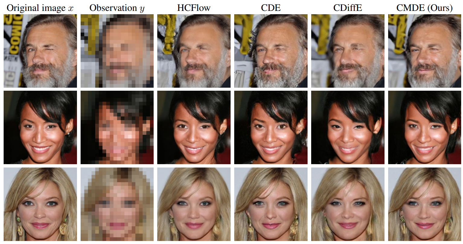
Experiments
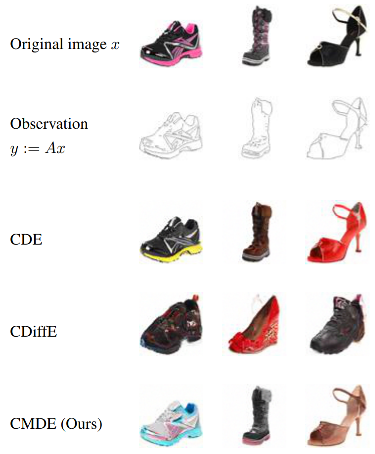
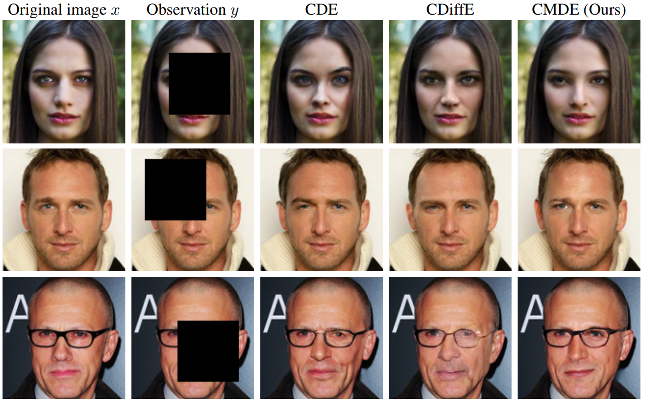
- 데이터셋: CelebA, Edges2shoes
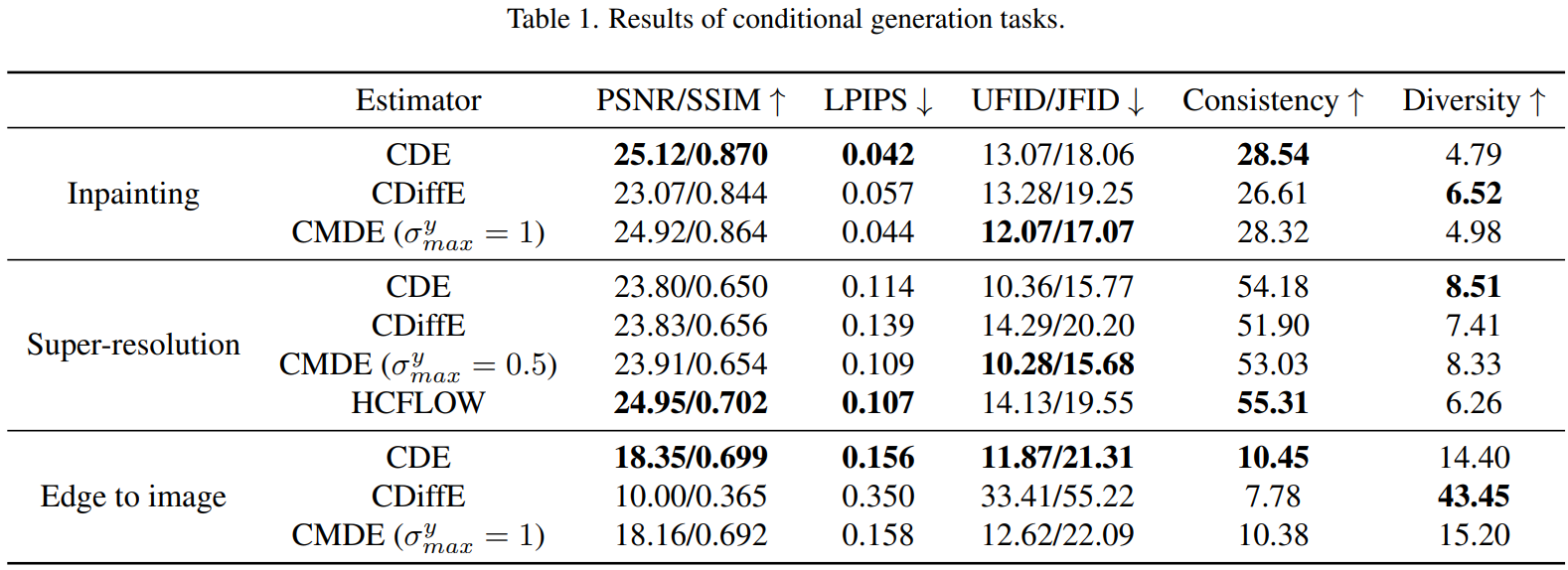
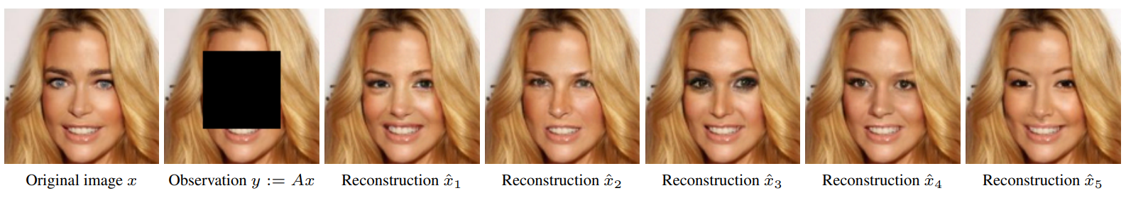
1. Inpainting
2. Super-resolution
3. Edge to image translation